4.5 Decision Rules

A decision rule is a simple IF-THEN statement consisting of a condition (also called antecedent) and a prediction. For example: IF it rains today AND if it is April (condition), THEN it will rain tomorrow (prediction). A single decision rule or a combination of several rules can be used to make predictions.

Decision rules follow a general structure: IF the conditions are met THEN make a certain prediction. Decision rules are probably the most interpretable prediction models. Their IF-THEN structure semantically resembles natural language and the way we think, provided that the condition is built from intelligible features, the length of the condition is short (small number of feature=value pairs combined with an AND) and there are not too many rules. In programming, it is very natural to write IF-THEN rules. New in machine learning is that the decision rules are learned through an algorithm.

Imagine using an algorithm to learn decision rules for predicting the value of a house (low, medium or high). One decision rule learned by this model could be: If a house is bigger than 100 square meters and has a garden, then its value is high. More formally: IF size>100 AND garden=1 THEN value=high.

Let us break down the decision rule:

• size>100 is the first condition in the IF-part.
• garden=1 is the second condition in the IF-part.
• The two conditions are connected with an 'AND' to create a new condition. Both must be true for the rule to apply.
• The predicted outcome (THEN-part) is value=high.

A decision rule uses at least one feature=value statement in the condition, with no upper limit on how many more can be added with an 'AND'. An exception is the default rule that has no explicit IF-part and that applies when no other rule applies, but more about this later.

The usefulness of a decision rule is usually summarized in two numbers: Support and accuracy.

Support or coverage of a rule: The percentage of instances to which the condition of a rule applies is called the support. Take for example the rule size=big AND location=good THEN value=high for predicting house values. Suppose 100 of 1000 houses are big and in a good location, then the support of the rule is 10%. The prediction (THEN-part) is not important for the calculation of support.

Accuracy or confidence of a rule: The accuracy of a rule is a measure of how accurate the rule is in predicting the correct class for the instances to which the condition of the rule applies. For example: Let us say of the 100 houses, where the rule size=big AND location=good THEN value=high applies, 85 have value=high, 14 have value=medium and 1 has value=low, then the accuracy of the rule is 85%.

Usually there is a trade-off between accuracy and support: By adding more features to the condition, we can achieve higher accuracy, but lose support.

To create a good classifier for predicting the value of a house you might need to learn not only one rule, but maybe 10 or 20. Then things can get more complicated and you can run into one of the following problems:

• Rules can overlap: What if I want to predict the value of a house and two or more rules apply and they give me contradictory predictions?
• No rule applies: What if I want to predict the value of a house and none of the rules apply?

There are two main strategies for combining multiple rules: Decision lists (ordered) and decision sets (unordered). Both strategies imply different solutions to the problem of overlapping rules.

A decision list introduces an order to the decision rules. If the condition of the first rule is true for an instance, we use the prediction of the first rule. If not, we go to the next rule and check if it applies and so on. Decision lists solve the problem of overlapping rules by only returning the prediction of the first rule in the list that applies.

A decision set resembles a democracy of the rules, except that some rules might have a higher voting power. In a set, the rules are either mutually exclusive, or there is a strategy for resolving conflicts, such as majority voting, which may be weighted by the individual rule accuracies or other quality measures. Interpretability suffers potentially when several rules apply.

Both decision lists and sets can suffer from the problem that no rule applies to an instance. This can be resolved by introducing a default rule. The default rule is the rule that applies when no other rule applies. The prediction of the default rule is often the most frequent class of the data points which are not covered by other rules. If a set or list of rules covers the entire feature space, we call it exhaustive. By adding a default rule, a set or list automatically becomes exhaustive.

There are many ways to learn rules from data and this book is far from covering them all. This chapter shows you three of them. The algorithms are chosen to cover a wide range of general ideas for learning rules, so all three of them represent very different approaches.

1. OneR learns rules from a single feature. OneR is characterized by its simplicity, interpretability and its use as a benchmark.
2. Sequential covering is a general procedure that iteratively learns rules and removes the data points that are covered by the new rule. This procedure is used by many rule learning algorithms.
3. Bayesian Rule Lists combine pre-mined frequent patterns into a decision list using Bayesian statistics. Using pre-mined patterns is a common approach used by many rule learning algorithms.

Let's start with the simplest approach: Using the single best feature to learn rules.

4.5.1 Learn Rules from a Single Feature (OneR)

The OneR algorithm suggested by Holte (1993)¹⁸ is one of the simplest rule induction algorithms. From all the features, OneR selects the one that carries the most information about the outcome of interest and creates decision rules from this feature.

Despite the name OneR, which stands for "One Rule", the algorithm generates more than one rule: It is actually one rule per unique feature value of the selected best feature. A better name would be OneFeatureRules.

The algorithm is simple and fast:

1. Discretize the continuous features by choosing appropriate intervals.
2. For each feature:
   • Create a cross table between the feature values and the (categorical) outcome.
   • For each value of the feature, create a rule which predicts the most frequent class of the instances that have this particular feature value (can be read from the cross table).
   • Calculate the total error of the rules for the feature.
3. Select the feature with the smallest total error.

OneR always covers all instances of the dataset, since it uses all levels of the selected feature. Missing values can be either treated as an additional feature value or be imputed beforehand.

A OneR model is a decision tree with only one split. The split is not necessarily binary as in CART, but depends on the number of unique feature values.

Let us look at an example how the best feature is chosen by OneR. The following table shows an artificial dataset about houses with information about its value, location, size and whether pets are allowed. We are interested in learning a simple model to predict the value of a house.

location	size	pets	value
good	small	yes	high
good	big	no	high
good	big	no	high
bad	medium	no	medium
good	medium	only cats	medium
good	small	only cats	medium
bad	medium	yes	medium
bad	small	yes	low
bad	medium	yes	low
bad	small	no	low

OneR creates the cross tables between each feature and the outcome:

	value=low	value=medium	value=high
location=bad	3	2	0
location=good	0	2	3

	value=low	value=medium	value=high
size=big	0	0	2
size=medium	1	3	0
size=small	2	1	1

	value=low	value=medium	value=high
pets=no	1	1	2
pets=only cats	0	2	0
pets=yes	2	1	1

For each feature, we go through the table row by row: Each feature value is the IF-part of a rule; the most common class for instances with this feature value is the prediction, the THEN-part of the rule. For example, the size feature with the levels small, medium and big results in three rules. For each feature we calculate the total error rate of the generated rules, which is the sum of the errors. The location feature has the possible values bad and good. The most frequent value for houses in bad locations is low and when we use low as a prediction, we make two mistakes, because two houses have a medium value. The predicted value of houses in good locations is high and again we make two mistakes, because two houses have a medium value. The error we make by using the location feature is 4/10, for the size feature it is 3/10 and for the pet feature it is 4/10 . The size feature produces the rules with the lowest error and will be used for the final OneR model:

IF size=small THEN value=small
IF size=medium THEN value=medium
IF size=big THEN value=high

OneR prefers features with many possible levels, because those features can overfit the target more easily. Imagine a dataset that contains only noise and no signal, which means that all features take on random values and have no predictive value for the target. Some features have more levels than others. The features with more levels can now more easily overfit. A feature that has a separate level for each instance from the data would perfectly predict the entire training dataset. A solution would be to split the data into training and validation sets, learn the rules on the training data and evaluate the total error for choosing the feature on the validation set.

Ties are another issue, i.e. when two features result in the same total error. OneR solves ties by either taking the first feature with the lowest error or the one with the lowest p-value of a chi-squared test.

Example

Let us try OneR with real data. We use the cervical cancer classification task to test the OneR algorithm. All continuous input features were discretized into their 5 quantiles. The following rules are created:

Age	prediction
(12.9,27.2]	Healthy
(27.2,41.4]	Healthy
(41.4,55.6]	Healthy
(55.6,69.8]	Healthy
(69.8,84.1]	Healthy

The age feature was chosen by OneR as the best predictive feature. Since cancer is rare, for each rule the majority class and therefore the predicted label is always Healthy, which is rather unhelpful. It does not make sense to use the label prediction in this unbalanced case. The cross table between the 'Age' intervals and Cancer/Healthy together with the percentage of women with cancer is more informative:

	# Cancer	# Healthy	P(Cancer)
Age=(12.9,27.2]	26	477	0.05
Age=(27.2,41.4]	25	290	0.08
Age=(41.4,55.6]	4	31	0.11
Age=(55.6,69.8]	0	1	0.00
Age=(69.8,84.1]	0	4	0.00

But before you start interpreting anything: Since the prediction for every feature and every value is Healthy, the total error rate is the same for all features. The ties in the total error are, by default, resolved by using the first feature from the ones with the lowest error rates (here, all features have 55/858), which happens to be the Age feature.

OneR does not support regression tasks. But we can turn a regression task into a classification task by cutting the continuous outcome into intervals. We use this trick to predict the number of rented bikes with OneR by cutting the number of bikes into its four quartiles (0-25%, 25-50%, 50-75% and 75-100%). The following table shows the selected feature after fitting the OneR model:

mnth	prediction
JAN	[22,3152]
FEB	[22,3152]
MAR	[22,3152]
APR	(3152,4548]
MAY	(5956,8714]
JUN	(4548,5956]
JUL	(5956,8714]
AUG	(5956,8714]
SEP	(5956,8714]
OKT	(5956,8714]
NOV	(3152,4548]
DEZ	[22,3152]

The selected feature is the month. The month feature has (surprise!) 12 feature levels, which is more than most other features have. So there is a danger of overfitting. On the more optimistic side: the month feature can handle the seasonal trend (e.g. less rented bikes in winter) and the predictions seem sensible.

Now we move from the simple OneR algorithm to a more complex procedure using rules with more complex conditions consisting of several features: Sequential Covering.

4.5.2 Sequential Covering

Sequential covering is a general procedure that repeatedly learns a single rule to create a decision list (or set) that covers the entire dataset rule by rule. Many rule-learning algorithms are variants of the sequential covering algorithm. This chapter introduces the main recipe and uses RIPPER, a variant of the sequential covering algorithm for the examples.

The idea is simple: First, find a good rule that applies to some of the data points. Remove all data points which are covered by the rule. A data point is covered when the conditions apply, regardless of whether the points are classified correctly or not. Repeat the rule-learning and removal of covered points with the remaining points until no more points are left or another stop condition is met. The result is a decision list. This approach of repeated rule-learning and removal of covered data points is called "separate-and-conquer".

Suppose we already have an algorithm that can create a single rule that covers part of the data. The sequential covering algorithm for two classes (one positive, one negative) works like this:

• Start with an empty list of rules (rlist).
• Learn a rule r.
• While the list of rules is below a certain quality threshold (or positive examples are not yet covered):
  • Add rule r to rlist.
  • Remove all data points covered by rule r.
  • Learn another rule on the remaining data.
• Return the decision list.

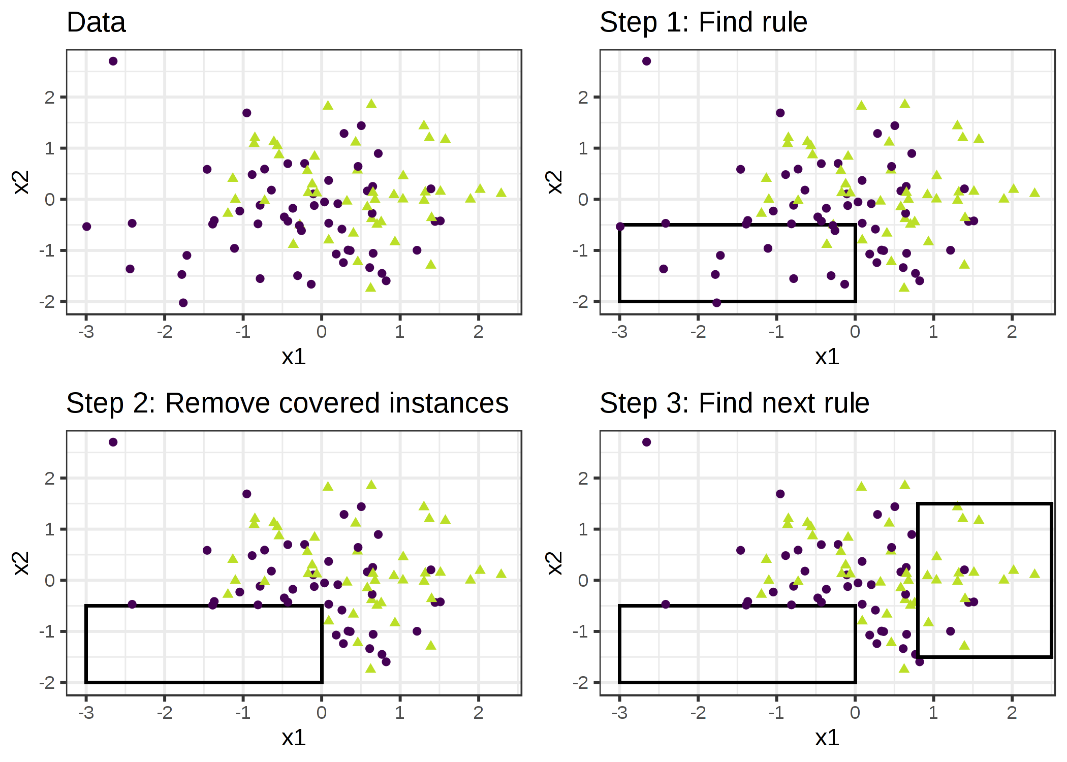
ภาพประกอบ 4.19: The covering algorithm works by sequentially covering the feature space with single rules and removing the data points that are already covered by those rules. For visualization purposes, the features x1 and x2 are continuous, but most rule learning algorithms require categorical features.

For example: We have a task and dataset for predicting the values of houses from size, location and whether pets are allowed. We learn the first rule, which turns out to be: If size=big and location=good, then value=high. Then we remove all big houses in good locations from the dataset. With the remaining data we learn the next rule. Maybe: If location=good, then value=medium. Note that this rule is learned on data without big houses in good locations, leaving only medium and small houses in good locations.

For multi-class settings, the approach must be modified. First, the classes are ordered by increasing prevalence. The sequential covering algorithm starts with the least common class, learns a rule for it, removes all covered instances, then moves on to the second least common class and so on. The current class is always treated as the positive class and all classes with a higher prevalence are combined in the negative class. The last class is the default rule. This is also referred to as one-versus-all strategy in classification.

How do we learn a single rule? The OneR algorithm would be useless here, since it would always cover the whole feature space. But there are many other possibilities. One possibility is to learn a single rule from a decision tree with beam search:

• Learn a decision tree (with CART or another tree learning algorithm).
• Start at the root node and recursively select the purest node (e.g. with the lowest misclassification rate).
• The majority class of the terminal node is used as the rule prediction; the path leading to that node is used as the rule condition.

The following figure illustrates the beam search in a tree:

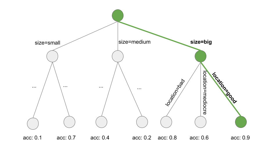
ภาพประกอบ 4.20: Learning a rule by searching a path through a decision tree. A decision tree is grown to predict the target of interest. We start at the root node, greedily and iteratively follow the path which locally produces the purest subset (e.g. highest accuracy) and add all the split values to the rule condition. We end up with: If location=good and size=big, then value=high.

Learning a single rule is a search problem, where the search space is the space of all possible rules. The goal of the search is to find the best rule according to some criteria. There are many different search strategies: hill-climbing, beam search, exhaustive search, best-first search, ordered search, stochastic search, top-down search, bottom-up search, ...

RIPPER (Repeated Incremental Pruning to Produce Error Reduction) by Cohen (1995)¹⁹ is a variant of the Sequential Covering algorithm. RIPPER is a bit more sophisticated and uses a post-processing phase (rule pruning) to optimize the decision list (or set). RIPPER can run in ordered or unordered mode and generate either a decision list or decision set.

Examples

We will use RIPPER for the examples.

The RIPPER algorithm does not find any rule in the classification task for cervical cancer.

When we use RIPPER on the regression task to predict bike counts some rules are found. Since RIPPER only works for classification, the bike counts must be turned into a categorical outcome. I achieved this by cutting the bike counts into the quartiles. For example (4548, 5956) is the interval covering predicted bike counts between 4548 and 5956. The following table shows the decision list of learned rules.

rules
(days_since_2011 >= 438) and (temp >= 17) and (temp <= 27) and (hum <= 67) => cnt=(5956,8714]
(days_since_2011 >= 443) and (temp >= 12) and (weathersit = GOOD) and (hum >= 59) => cnt=(5956,8714]
(days_since_2011 >= 441) and (windspeed <= 10) and (temp >= 13) => cnt=(5956,8714]
(temp >= 12) and (hum <= 68) and (days_since_2011 >= 551) => cnt=(5956,8714]
(days_since_2011 >= 100) and (days_since_2011 <= 434) and (hum <= 72) and (workingday = WORKING DAY) => cnt=(3152,4548]
(days_since_2011 >= 106) and (days_since_2011 <= 323) => cnt=(3152,4548]
=> cnt=[22,3152]

The interpretation is simple: If the conditions apply, we predict the interval on the right hand side for the number of bikes. The last rule is the default rule that applies when none of the other rules apply to an instance. To predict a new instance, start at the top of the list and check whether a rule applies. When a condition matches, then the right hand side of the rule is the prediction for this instance. The default rule ensures that there is always a prediction.

4.5.3 Bayesian Rule Lists

In this section, I will show you another approach to learning a decision list, which follows this rough recipe:

1. Pre-mine frequent patterns from the data that can be used as conditions for the decision rules.
2. Learn a decision list from a selection of the pre-mined rules.

A specific approach using this recipe is called Bayesian Rule Lists (Letham et. al, 2015)²⁰ or BRL for short. BRL uses Bayesian statistics to learn decision lists from frequent patterns which are pre-mined with the FP-tree algorithm (Borgelt 2005)²¹

But let us start slowly with the first step of BRL.

Pre-mining of frequent patterns

A frequent pattern is the frequent (co-)occurrence of feature values. As a pre-processing step for the BRL algorithm, we use the features (we do not need the target outcome in this step) and extract frequently occurring patterns from them. A pattern can be a single feature value such as size=medium or a combination of feature values such as size=medium AND location=bad.

The frequency of a pattern is measured with its support in the dataset:

\[Support(x_j=A)=\frac{1}n{}\sum_{i=1}^nI(x^{(i)}_{j}=A)\]

where A is the feature value, n the number of data points in the dataset and I the indicator function that returns 1 if the feature \(x_j\) of the instance i has level A otherwise 0. In a dataset of house values, if 20% of houses have no balcony and 80% have one or more, then the support for the pattern balcony=0 is 20%. Support can also be measured for combinations of feature values, for example for balcony=0 AND pets=allowed.

There are many algorithms to find such frequent patterns, for example Apriori or FP-Growth. Which you use does not matter much, only the speed at which the patterns are found is different, but the resulting patterns are always the same.

I will give you a rough idea of how the Apriori algorithm works to find frequent patterns. Actually the Apriori algorithm consists of two parts, where the first part finds frequent patterns and the second part builds association rules from them. For the BRL algorithm, we are only interested in the frequent patterns that are generated in the first part of Apriori.

In the first step, the Apriori algorithm starts with all feature values that have a support greater than the minimum support defined by the user. If the user says that the minimum support should be 10% and only 5% of the houses have size=big, we would remove that feature value and keep only size=medium and size=small as patterns. This does not mean that the houses are removed from the data, it just means that size=big is not returned as frequent pattern. Based on frequent patterns with a single feature value, the Apriori algorithm iteratively tries to find combinations of feature values of increasingly higher order. Patterns are constructed by combining feature=value statements with a logical AND, e.g. size=medium AND location=bad. Generated patterns with a support below the minimum support are removed. In the end we have all the frequent patterns. Any subset of a frequent pattern is frequent again, which is called the Apriori property. It makes sense intuitively: By removing a condition from a pattern, the reduced pattern can only cover more or the same number of data points, but not less. For example, if 20% of the houses are size=medium and location=good, then the support of houses that are only size=medium is 20% or greater. The Apriori property is used to reduce the number of patterns to be inspected. Only in the case of frequent patterns we have to check patterns of higher order.

Now we are done with pre-mining conditions for the Bayesian Rule List algorithm. But before we move on to the second step of BRL, I would like to hint at another way for rule-learning based on pre-mined patterns. Other approaches suggest including the outcome of interest into the frequent pattern mining process and also executing the second part of the Apriori algorithm that builds IF-THEN rules. Since the algorithm is unsupervised, the THEN-part also contains feature values we are not interested in. But we can filter by rules that have only the outcome of interest in the THEN-part. These rules already form a decision set, but it would also be possible to arrange, prune, delete or recombine the rules.

In the BRL approach however, we work with the frequent patterns and learn the THEN-part and how to arrange the patterns into a decision list using Bayesian statistics.

Learning Bayesian Rule Lists

The goal of the BRL algorithm is to learn an accurate decision list using a selection of the pre-mined conditions, while prioritizing lists with few rules and short conditions. BRL addresses this goal by defining a distribution of decision lists with prior distributions for the length of conditions (preferably shorter rules) and the number of rules (preferably a shorter list).

The posteriori probability distribution of lists makes it possible to say how likely a decision list is, given assumptions of shortness and how well the list fits the data. Our goal is to find the list that maximizes this posterior probability. Since it is not possible to find the exact best list directly from the distributions of lists, BRL suggests the following recipe:
1) Generate an initial decision list, which is randomly drawn from the priori distribution.
2) Iteratively modify the list by adding, switching or removing rules, ensuring that the resulting lists follow the posterior distribution of lists.
3) Select the decision list from the sampled lists with the highest probability according to the posteriori distribution.

Let us go over the algorithm more closely: The algorithm starts with pre-mining feature value patterns with the FP-Growth algorithm. BRL makes a number of assumptions about the distribution of the target and the distribution of the parameters that define the distribution of the target. (That's Bayesian statistic.) If you are unfamiliar with Bayesian statistics, do not get too caught up in the following explanations. It is important to know that the Bayesian approach is a way to combine existing knowledge or requirements (so-called priori distributions) while also fitting to the data. In the case of decision lists, the Bayesian approach makes sense, since the prior assumptions nudges the decision lists to be short with short rules.

The goal is to sample decision lists d from the posteriori distribution:

\[\underbrace{p(d|x,y,A,\alpha,\lambda,\eta)}_{posteriori}\propto\underbrace{p(y|x,d,\alpha)}_{likelihood}\cdot\underbrace{p(d|A,\lambda,\eta)}_{priori}\]

where d is a decision list, x are the features, y is the target, A the set of pre-mined conditions, \(\lambda\) the prior expected length of the decision lists, \(\eta\) the prior expected number of conditions in a rule, \(\alpha\) the prior pseudo-count for the positive and negative classes which is best fixed at (1,1).

\[p(d|x,y,A,\alpha,\lambda,\eta)\]

quantifies how probable a decision list is, given the observed data and the priori assumptions. This is proportional to the likelihood of the outcome y given the decision list and the data times the probability of the list given prior assumptions and the pre-mined conditions.

\[p(y|x,d,\alpha)\]

is the likelihood of the observed y, given the decision list and the data. BRL assumes that y is generated by a Dirichlet-Multinomial distribution. The better the decision list d explains the data, the higher the likelihood.

\[p(d|A,\lambda,\eta)\]

is the prior distribution of the decision lists. It multiplicatively combines a truncated Poisson distribution (parameter \(\lambda\)) for the number of rules in the list and a truncated Poisson distribution (parameter \(\eta\)) for the number of feature values in the conditions of the rules.

A decision list has a high posterior probability if it explains the outcome y well and is also likely according to the prior assumptions.

Estimations in Bayesian statistics are always a bit tricky, because we usually cannot directly calculate the correct answer, but we have to draw candidates, evaluate them and update our posteriori estimates using the Markov chain Monte Carlo method. For decision lists, this is even more tricky, because we have to draw from the distribution of decision lists. The BRL authors propose to first draw an initial decision list and then iteratively modify it to generate samples of decision lists from the posterior distribution of the lists (a Markov chain of decision lists). The results are potentially dependent on the initial decision list, so it is advisable to repeat this procedure to ensure a great variety of lists. The default in the software implementation is 10 times. The following recipe tells us how to draw an initial decision list:

• Pre-mine patterns with FP-Growth.
• Sample the list length parameter m from a truncated Poisson distribution.
• For the default rule: Sample the Dirichlet-Multinomial distribution parameter \(\theta_0\) of the target value (i.e. the rule that applies when nothing else applies).
• For decision list rule j=1,...,m, do:
  • Sample the rule length parameter l (number of conditions) for rule j.
  • Sample a condition of length \(l_j\) from the pre-mined conditions.
  • Sample the Dirichlet-Multinomial distribution parameter for the THEN-part (i.e. for the distribution of the target outcome given the rule)
• For each observation in the dataset:
  • Find the rule from the decision list that applies first (top to bottom).
  • Draw the predicted outcome from the probability distribution (Binomial) suggested by the rule that applies.

The next step is to generate many new lists starting from this initial sample to obtain many samples from the posterior distribution of decision lists.

The new decision lists are sampled by starting from the initial list and then randomly either moving a rule to a different position in the list or adding a rule to the current decision list from the pre-mined conditions or removing a rule from the decision list. Which of the rules is switched, added or deleted is chosen at random. At each step, the algorithm evaluates the posteriori probability of the decision list (mixture of accuracy and shortness). The Metropolis Hastings algorithm ensures that we sample decision lists that have a high posterior probability. This procedure provides us with many samples from the distribution of decision lists. The BRL algorithm selects the decision list of the samples with the highest posterior probability.

Examples

That is it with the theory, now let's see the BRL method in action. The examples use a faster variant of BRL called Scalable Bayesian Rule Lists (SBRL) by Yang et. al (2017) ²². We use the SBRL algorithm to predict the risk for cervical cancer. I first had to discretize all input features for the SBRL algorithm to work. For this purpose I binned the continuous features based on the frequency of the values by quantiles.

We get the following rules:

rules
If {STDs=1} (rule[259]) then positive probability = 0.16049383
else if {Hormonal.Contraceptives..years.=[0,10)} (rule[82]) then positive probability = 0.04685408
else (default rule) then positive probability = 0.27777778

Note that we get sensible rules, since the prediction on the THEN-part is not the class outcome, but the predicted probability for cancer.

The conditions were selected from patterns that were pre-mined with the FP-Growth algorithm. The following table displays the pool of conditions the SBRL algorithm could choose from for building a decision list. The maximum number of feature values in a condition I allowed as a user was two. Here is a sample of ten patterns:

pre-mined conditions
Num.of.pregnancies=[3.67,7.33)
IUD=0,STDs=1
Number.of.sexual.partners=[1,10),STDs..Time.since.last.diagnosis=[1,8)
First.sexual.intercourse=[10,17.3),STDs=0
Smokes=1,IUD..years.=[0,6.33)
Hormonal.Contraceptives..years.=[10,20),STDs..Number.of.diagnosis=[0,1)
Age=[13,36.7)
Hormonal.Contraceptives=1,STDs..Number.of.diagnosis=[0,1)
Number.of.sexual.partners=[1,10),STDs..number.=[0,1.33)
STDs..number.=[1.33,2.67),STDs..Time.since.first.diagnosis=[1,8)

Next, we apply the SBRL algorithm to the bike rental prediction task. This only works if the regression problem of predicting bike counts is converted into a binary classification task. I have arbitrarily created a classification task by creating a label that is 1 if the number of bikes exceeds 4000 bikes on a day, else 0.

The following list was learned by SBRL:

rules
If {yr=2011,temp=[-5.22,7.35)} (rule[718]) then positive probability = 0.01041667
else if {yr=2012,temp=[7.35,19.9)} (rule[823]) then positive probability = 0.88125000
else if {yr=2012,temp=[19.9,32.5]} (rule[816]) then positive probability = 0.99253731
else if {season=SPRING} (rule[351]) then positive probability = 0.06410256
else if {temp=[7.35,19.9)} (rule[489]) then positive probability = 0.44444444
else (default rule) then positive probability = 0.79746835

Let us predict the probability that the number of bikes will exceed 4000 for a day in 2012 with a temperature of 17 degrees Celsius. The first rule does not apply, since it only applies for days in 2011. The second rule applies, because the day is in 2012 and 17 degrees lies in the interval [7.35,19.9). Our prediction for the probability is that more than 4000 bikes are rented is 88%.

4.5.4 Advantages

This section discusses the benefits of IF-THEN rules in general.

IF-THEN rules are easy to interpret. They are probably the most interpretable of the interpretable models. This statement only applies if the number of rules is small, the conditions of the rules are short (maximum 3 I would say) and if the rules are organized in a decision list or a non-overlapping decision set.

Decision rules can be as expressive as decision trees, while being more compact. Decision trees often also suffer from replicated sub-trees, that is, when the splits in a left and a right child node have the same structure.

The prediction with IF-THEN rules is fast, since only a few binary statements need to be checked to determine which rules apply.

Decision rules are robust against monotonic transformations of the input features, because only the threshold in the conditions changes. They are also robust against outliers, since it only matters if a condition applies or not.

IF-THEN rules usually generate sparse models, which means that not many features are included. They select only the relevant features for the model. For example, a linear model assigns a weight to every input feature by default. Features that are irrelevant can simply be ignored by IF-THEN rules.

Simple rules like from OneR can be used as baseline for more complex algorithms.

4.5.5 Disadvantages

This section deals with the disadvantages of IF-THEN rules in general.

The research and literature for IF-THEN rules focuses on classification and almost completely neglects regression. While you can always divide a continuous target into intervals and turn it into a classification problem, you always lose information. In general, approaches are more attractive if they can be used for both regression and classification.

Often the features also have to be categorical. That means numeric features must be categorized if you want to use them. There are many ways to cut a continuous feature into intervals, but this is not trivial and comes with many questions without clear answers. How many intervals should the feature be divided into? What is the splitting criteria: Fixed interval lengths, quantiles or something else? Categorizing continuous features is a non-trivial issue that is often neglected and people just use the next best method (like I did in the examples).

Many of the older rule-learning algorithms are prone to overfitting. The algorithms presented here all have at least some safeguards to prevent overfitting: OneR is limited because it can only use one feature (only problematic if the feature has too many levels or if there are many features, which equates to the multiple testing problem), RIPPER does pruning and Bayesian Rule Lists impose a prior distribution on the decision lists.

Decision rules are bad in describing linear relationships between features and output. That is a problem they share with the decision trees. Decision trees and rules can only produce step-like prediction functions, where changes in the prediction are always discrete steps and never smooth curves. This is related to the issue that the inputs have to be categorical. In decision trees, they are implicitly categorized by splitting them.

4.5.6 Software and Alternatives

OneR is implemented in the R package OneR, which was used for the examples in this book. OneR is also implemented in the Weka machine learning library and as such available in Java, R and Python. RIPPER is also implemented in Weka. For the examples, I used the R implementation of JRIP in the RWeka package. SBRL is available as R package (which I used for the examples), in Python or as C implementation.

I will not even try to list all alternatives for learning decision rule sets and lists, but will point to some summarizing work. I recommend the book "Foundations of Rule Learning" by Fuernkranz et. al (2012)²³. It is an extensive work on learning rules, for those who want to delve deeper into the topic. It provides a holistic framework for thinking about learning rules and presents many rule learning algorithms. I also recommend to checkout the Weka rule learners, which implement RIPPER, M5Rules, OneR, PART and many more. IF-THEN rules can be used in linear models as described in this book in the chapter about the RuleFit algorithm.

---

18. Holte, Robert C. "Very simple classification rules perform well on most commonly used datasets." Machine learning 11.1 (1993): 63-90.↩

19. Cohen, William W. "Fast effective rule induction." Machine Learning Proceedings (1995). 115-123.↩

20. Letham, Benjamin, et al. "Interpretable classifiers using rules and Bayesian analysis: Building a better stroke prediction model." The Annals of Applied Statistics 9.3 (2015): 1350-1371.↩

21. Borgelt, C. "An implementation of the FP-growth algorithm." Proceedings of the 1st International Workshop on Open Source Data Mining Frequent Pattern Mining Implementations - OSDM ’05, 1–5. http://doi.org/10.1145/1133905.1133907 (2005).↩

22. Yang, Hongyu, Cynthia Rudin, and Margo Seltzer. "Scalable Bayesian rule lists." Proceedings of the 34th International Conference on Machine Learning-Volume 70. JMLR. org, 2017.↩

23. Fürnkranz, Johannes, Dragan Gamberger, and Nada Lavrač. "Foundations of rule learning." Springer Science & Business Media, (2012).↩