6.1 Counterfactual Explanations

Authors: Susanne Dandl & Christoph Molnar

A counterfactual explanation describes a causal situation in the form: "If X had not occurred, Y would not have occurred". For example: "If I hadn't taken a sip of this hot coffee, I wouldn't have burned my tongue". Event Y is that I burned my tongue; cause X is that I had a hot coffee. Thinking in counterfactuals requires imagining a hypothetical reality that contradicts the observed facts (for example, a world in which I have not drunk the hot coffee), hence the name "counterfactual". The ability to think in counterfactuals makes us humans so smart compared to other animals.

In interpretable machine learning, counterfactual explanations can be used to explain predictions of individual instances. The "event" is the predicted outcome of an instance, the "causes" are the particular feature values of this instance that were input to the model and "caused" a certain prediction. Displayed as a graph, the relationship between the inputs and the prediction is very simple: The feature values cause the prediction.

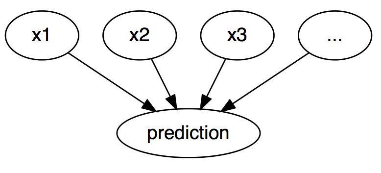
ภาพประกอบ 6.1: The causal relationships between inputs of a machine learning model and the predictions, when the model is merely seen as a black box. The inputs cause the prediction (not necessarily reflecting the real causal relation of the data).

Even if in reality the relationship between the inputs and the outcome to be predicted might not be causal, we can see the inputs of a model as the cause of the prediction.

Given this simple graph, it is easy to see how we can simulate counterfactuals for predictions of machine learning models: We simply change the feature values of an instance before making the predictions and we analyze how the prediction changes. We are interested in scenarios in which the prediction changes in a relevant way, like a flip in predicted class (for example, credit application accepted or rejected) or in which the prediction reaches a certain threshold (for example, the probability for cancer reaches 10%). A counterfactual explanation of a prediction describes the smallest change to the feature values that changes the prediction to a predefined output.

There are both model-agnostic and model-specific counterfactual explanation methods, but in this chapter we focus on model-agnostic methods that only work with the model inputs and outputs (and not the internal structure of specific models). These methods would also feel at home in the model-agnostic chapter, since the interpretation can be expressed as a summary of the differences in feature values ("change features A and B to change the prediction"). But a counterfactual explanation is itself a new instance, so it lives in this chapter ("starting from instance X, change A and B to get a counterfactual instance"). Unlike prototypes, counterfactuals do not have to be actual instances from the training data, but can be a new combination of feature values.

Before discussing how to create counterfactuals, I would like to discuss some use cases for counterfactuals and how a good counterfactual explanation looks like.

In this first example, Peter applies for a loan and gets rejected by the (machine learning powered) banking software. He wonders why his application was rejected and how he might improve his chances to get a loan. The question of "why" can be formulated as a counterfactual: What is the smallest change to the features (income, number of credit cards, age, ...) that would change the prediction from rejected to approved? One possible answer could be: If Peter would earn 10,000 Euro more per year, he would get the loan. Or if Peter had fewer credit cards and had not defaulted on a loan 5 years ago, he would get the loan. Peter will never know the reasons for the rejection, as the bank has no interest in transparency, but that is another story.

In our second example we want to explain a model that predicts a continuous outcome with counterfactual explanations. Anna wants to rent out her apartment, but she is not sure how much to charge for it, so she decides to train a machine learning model to predict the rent. Of course, since Anna is a data scientist, that is how she solves her problems. After entering all the details about size, location, whether pets are allowed and so on, the model tells her that she can charge 900 Euro. She expected 1000 Euro or more, but she trusts her model and decides to play with the feature values of the apartment to see how she can improve the value of the apartment. She finds out that the apartment could be rented out for over 1000 Euro, if it were 15 m² larger. Interesting, but non-actionable knowledge, because she cannot enlarge her apartment. Finally, by tweaking only the feature values under her control (built-in kitchen yes/no, pets allowed yes/no, type of floor, etc.), she finds out that if she allows pets and installs windows with better insulation, she can charge 1000 Euro. Anna had intuitively worked with counterfactuals to change the outcome.

Counterfactuals are human-friendly explanations, because they are contrastive to the current instance and because they are selective, meaning they usually focus on a small number of feature changes. But counterfactuals suffer from the 'Rashomon effect'. Rashomon is a Japanese movie in which the murder of a Samurai is told by different people. Each of the stories explains the outcome equally well, but the stories contradict each other. The same can also happen with counterfactuals, since there are usually multiple different counterfactual explanations. Each counterfactual tells a different "story" of how a certain outcome was reached. One counterfactual might say to change feature A, the other counterfactual might say to leave A the same but change feature B, which is a contradiction. This issue of multiple truths can be addressed either by reporting all counterfactual explanations or by having a criterion to evaluate counterfactuals and select the best one.

Speaking of criteria, how do we define a good counterfactual explanation? First, the user of a counterfactual explanation defines a relevant change in the prediction of an instance (= the alternative reality). An obvious first requirement is that a counterfactual instance produces the predefined prediction as closely as possible. It is not always possible to find a counterfactual with the predefined prediction. For example, in a classification setting with two classes, a rare class and a frequent class, the model might always classify an instance as the frequent class. Changing the feature values so that the predicted label would flip from the frequent class to the rare class might be impossible. We want therfore relax the requirement that the prediction of the counterfactual must exactly match the predefined outcome. In the classification example, we could look for a counterfactual where the predicted probability of the rare class is increased to 10% instead of the current 2%. The question then is, what are the minimal changes in the features so that the predicted probability changes from 2% to 10% (or close to 10%)? Another quality criterion is that a counterfactual should be as similar as possible to the instance regarding feature values. The distance between two instances can be measured, for example, with the Manhattan distance or the Gower distance if we have both discrete and continuous features. The counterfactual should not only be close to the original instance, but should also change as few features as possible. To measure how good a counterfactual explanation is in this metric, we can simply count the number of changed features or, in fancy mathematical terms, measure the \(L_0\) norm between counterfactual and actual instance. Third, it is often desirable to generate multiple diverse counterfactual explanations so that the decision-subject gets access to multiple viable ways of generating a different outcome. For instance, continuing our loan example, one counterfactual explanation might suggest only to double the income to get a loan, while another counterfactual might suggest shifting to a nearby city and increase the income by a small amount to get a loan. It could be noted that while the first counterfactual might be possible for some, the latter might be more actionable for some. Thus, besides providing a decision-subject with different ways to get the desired outcome, diversity also enables "diverse" individuals to alter the features that are convenient for them. The last requirement is that a counterfactual instance should have feature values that are likely. It would not make sense to generate a counterfactual explanation for the rent example where the size of an apartment is negative or the number of rooms is set to 200. It is even better when the counterfactual is likely according to the joint distribution of the data, for example, an apartment with 10 rooms and 20 m² should not be regarded as counterfactual explanation. Ideally, if the number of square meters is increased, an increase in the number of rooms should also be proposed.

6.1.1 Generating Counterfactual Explanations

A simple and naive approach to generating counterfactual explanations is searching by trial and error. This approach involves randomly changing feature values of the instance of interest and stopping when the desired output is predicted. Like the example where Anna tried to find a version of her apartment for which she could charge more rent. But there are better approaches than trial and error. First, we define a loss function based on the criteria mentioned above. This loss takes as input the instance of interest, a counterfactual and the desired (counterfactual) outcome. Then, we can find the counterfactual explanation that minimizes this loss using an optimization algorithm. Many methods proceed in this way but differ in their definition of the loss function and optimization method.

In the following, we focus on two of them: first, the one by Wachter et. al (2017)⁵⁵ who introduced counterfactual explanation as an interpretation method and, second, the one by Dandl et al. (2020)⁵⁶ that takes into account all four criteria mentioned above.

6.1.1.1 Method by Wachter et al.

Wachter et al. suggest minimizing the following loss:

\[L(x,x^\prime,y^\prime,\lambda)=\lambda\cdot(\hat{f}(x^\prime)-y^\prime)^2+d(x,x^\prime)\]

The first term is the quadratic distance between the model prediction for the counterfactual x' and the desired outcome y', which the user must define in advance. The second term is the distance d between the instance x to be explained and the counterfactual x'. The loss measures how far the predicted outcome of the counterfactual is from the predefined outcome and how far the counterfactual is from the instance of interest. The distance function d is defined as the Manhattan distance weighted with the inverse median absolute deviation (MAD) of each feature.

\[d(x,x^\prime)=\sum_{j=1}^p\frac{|x_j-x^\prime_j|}{MAD_j}\]

The total distance is the sum of all p feature-wise distances, that is, the absolute differences of feature values between instance x and counterfactual x'. The feature-wise distances are scaled by the inverse of the median absolute deviation of feature j over the dataset defined as:

\[MAD_j=\text{median}_{i\in{}\{1,\ldots,n\}}(|x_{i,j}-\text{median}_{l\in{}\{1,\ldots,n\}}(x_{l,j})|)\]

The median of a vector is the value at which half of the vector values are greater and the other half smaller. The MAD is the equivalent of the variance of a feature, but instead of using the mean as the center and summing over the square distances, we use the median as the center and sum over the absolute distances. The proposed distance function has the advantage over the Euclidean distance that it is more robust to outliers. Scaling with the MAD is necessary to bring all the features to the same scale - it should not matter whether you measure the size of an apartment in square meters or square feet.

The parameter \(\lambda\) balances the distance in prediction (first term) against the distance in feature values (second term). The loss is solved for a given \(\lambda\) and returns a counterfactual x'. A higher value of \(\lambda\) means that we prefer counterfactuals with predictions close to the desired outcome y', a lower value means that we prefer counterfactuals x' that are very similar to x in the feature values. If \(\lambda\) is very large, the instance with the prediction closest to y' will be selected, regardless how far it is away from x. Ultimately, the user must decide how to balance the requirement that the prediction for the counterfactual matches the desired outcome with the requirement that the counterfactual is similar to x. The authors of the method suggest instead of selecting a value for \(\lambda\) to select a tolerance \(\epsilon\) for how far away the prediction of the counterfactual instance is allowed to be from y'. This constraint can be written as:

\[|\hat{f}(x^\prime)-y^\prime|\leq\epsilon\]

To minimize this loss function, any suitable optimization algorithm can be used, such as Nelder-Mead. If you have access to the gradients of the machine learning model, you can use gradient-based methods like ADAM. The instance x to be explained, the desired output y' and the tolerance parameter \(\epsilon\) must be set in advance. The loss function is minimized for x' and the (locally) optimal counterfactual x' returned while increasing \(\lambda\) until a sufficiently close solution is found (= within the tolerance parameter):

\[\arg\min_{x^\prime}\max_{\lambda}L(x,x^\prime,y^\prime,\lambda).\]

Overall, the recipe for producing the counterfactuals is simple:

1. Select an instance x to be explained, the desired outcome y', a tolerance \(\epsilon\) and a (low) initial value for \(\lambda\).
2. Sample a random instance as initial counterfactual.
3. Optimize the loss with the initially sampled counterfactual as starting point.
4. While \(|\hat{f}(x^\prime)-y^\prime|>\epsilon\):
   • Increase \(\lambda\).
   • Optimize the loss with the current counterfactual as starting point.
   • Return the counterfactual that minimizes the loss.
5. Repeat steps 2-4 and return the list of counterfactuals or the one that minimizes the loss.

The proposed method has some disadvantages. It only takes the first and second criteria into account not the last two ("produce counterfactuals with only a few feature changes and likely feature values"). d does not prefer sparse solutions since increasing 10 features by 1 will give the same distance to x as increasing one feature by 10. Unrealistic feature combinations are not penalized.

The method does not handle categorical features with many different levels well. The authors of the method suggested running the method separately for each combination of feature values of the categorical features, but this will lead to a combinatorial explosion if you have multiple categorical features with many values. For example, 6 categorical features with 10 unique levels would mean 1 million runs.

Let us now have a look on another approach overcoming these issues.

6.1.1.2 Method by Dandl et al.

Dandl et al. suggest to simultaneously minimize a four-objective loss:

\[L(x,x',y',X^{obs})=\big(o_1(\hat{f}(x'),y'),o_2(x, x'),o_3(x,x'),o_4(x',X^{obs})\big) \]

Each of the four objectives \(o_1\) to \(o_4\) corresponds to one of the four criteria mentioned above. The first objective \(o_1\) reflects that the prediction of our counterfactual x' should be as close as possible to our desired prediction y'. We therefore want to minimize the distance between \(\hat{f}(x')\) and y', here calculated by the Manhattan metric (\(L_1\) norm):

\[o_1(\hat{f}(x'),y')=\begin{cases}0&\text{if $\hat{f}(x')\in{}y'$}\\\inf\limits_{y'\in y'}|\hat{f}(x')-y'|&\text{else}\end{cases}\]

The second objective \(o_2\) reflects that our counterfactual should be as similar as possible to our instance \(x\). It quantifies the distance between x' and x as the Gower distance:

\[o_2(x,x')=\frac{1}{p}\sum_{j=1}^{p}\delta_G(x_j, x'_j)\]

with p being the number of features. The value of \(\delta_G\) depends on the feature type of \(x_j\):

\[\delta_G(x_j,x'_j)=\begin{cases}\frac{1}{\widehat{R}_j}|x_j-x'_j|&\text{if $x_j$ numerical}\\\mathbb{I}_{x_j\neq{}x'_j}&\text{if $x_j$ categorical}\end{cases}\]

Dividing the distance of a numeric feature \(j\) by \(\widehat{R}_j\), the observed value range, scales \(\delta_G\) for all features between 0 and 1.

The Gower distance can handle both numerical and categorical features but does not count how many features were changed. Therefore, we count the number of features in a third objectives \(o_3\) using the \(L_0\) norm:

\[o_3(x,x')=||x-x'||_0=\sum_{j=1}^{p}\mathbb{I}_{x'_j\neq x_j}.\]

By minimizing \(o_3\) we aim for our third criteria - sparse feature changes.

The fourth objective \(o_4\) reflects that our counterfactuals should have likely feature values/combinations. We can infer how "likely" a data point is using the training data or another dataset. We denote this dataset as \(X^{obs}\). As an approximation for the likelihood, \(o_4\) measures the average Gower distance between x' and the nearest observed data point \(x^{[1]}\in{}X^{obs}\):

\[o_4(x',\textbf{X}^{obs})=\frac{1}{p}\sum_{j=1}^{p}\delta_G(x'_j,x^{[1]}_j)\]

Compared to Wachter et al., \(L(x,x',y',X^{obs})\) has no balancing/weighting terms like \(\lambda\). We do not want to collapse the four objectives \(o_1\), \(o_2\), \(o_3\) and \(o_4\) into a single objective by summing them up and weighting them, but we want to optimize all four terms simultaneously.

How can we do that? We use the Nondominated Sorting Genetic Algorithm⁵⁷ or short NSGA-II. NSGA-II is a nature-inspired algorithm that applies Darwin's law of the "survival of the fittest". We denote the fitness of a counterfactual by its vector of objectives values \((o_1,o_2,o_3,o_4)\). The lower a counterfactuals four objectives, the "fitter" it is.

The algorithm consists of four steps that are repeated until a stopping criterion is met, for example, a maximum number of iterations/generations. The following figure visualizes the four steps of one generation.

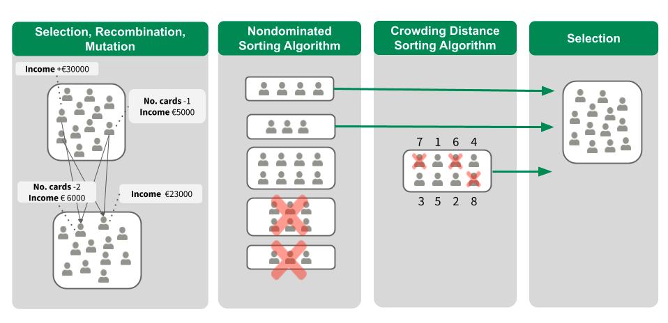
ภาพประกอบ 6.2: Visualization of one generation of the NSGA-II algorithm.

In the first generation a group of counterfactual candidates is initialized by randomly changing some of the features compared to our instance x to be explained. Sticking with above's credit example, one counterfactual could suggest to increase the income by € 30,000 while another one proposes to have no default in the last 5 years and a reduction in age by 10. All other feature values are equal to the values of x. Each candidate is then evaluated using the four objective functions of above. Among them, we randomly select some candidates, where fitter candidates are more likely selected. The candidates are pairwise recombined to produce children that are similar to them by averaging their numerical feature values or by crossing over their categorical features. In addition, we slightly mutate the feature values of the children to explore the whole feature space.

From the two resulting groups, one with parents and one with children, we only want the best half using two sorting algorithms. The nondominated sorting algorithm sorts the candidates according to their objective values. If candidates are equally good, the crowding distance sorting algorithm sorts the candidates according to their diversity.

Given the ranking of the two sorting algorithms, we select the most promising and/or most diverse half of the candidates. We use this set for the next generation and start again with the selection, recombination and mutation process. By repeating the steps over and over we hopefully approach a diverse set of promising candidates with low objective values. From this set we can choose those with which we are most satisfied, or we can give a summary of all counterfactuals by highlighting which and how often features have been changed.

6.1.2 Example

The following example is based on the credit dataset example in Dandl et al. (2020). The German Credit Risk dataset can be found on the machine learning challenges platform kaggle.com.

The authors trained a support vector machine (with radial basis kernel) to predict the probability that a costumer has a good credit risk. The corresponding dataset has 522 complete observations and nine features containing credit and customer information.

The goal is to find counterfactual explanations for a customer with the following feature values

age	sex	job	housing	savings	checking	amount	duration	purpose
58	f	unskilled	free	little	little	6143	48	car

The SVM predicts that the woman has a good credit risk with a probability of 24.2 %. The counterfactuals should answer how the input features need to be changed to get a predicted probability larger than 50 %?

The following table shows the 10 best counterfactuals:

age	sex	job	amount	duration	\(o_2\)	\(o_3\)	\(o_3\)	\(\hat{f}(x')\)
		skilled		-20	0.108	2	0.036	0.501
		skilled		-24	0.114	2	0.029	0.525
		skilled		-22	0.111	2	0.033	0.513
-6		skilled		-24	0.126	3	0.018	0.505
-3		skilled		-24	0.120	3	0.024	0.515
-1		skilled		-24	0.116	3	0.027	0.522
-3	m			-24	0.195	3	0.012	0.501
-6	m			-25	0.202	3	0.011	0.501
-30	m	skilled		-24	0.285	4	0.005	0.590
-4	m		-1254	-24	0.204	4	0.002	0.506

The first five columns contain the proposed feature changes (only altered features are displayed), the next three columns show the objective values (\(o_1\) equals 0 in all cases) and the last column displays the predicted probability.

All counterfactuals have predicted probabilities greater than 50 % and do not dominate each other. Nondominated means that none of the counterfactuals has smaller values in all objectives than the other counterfactuals. We can think of our counterfactuals as a set of trade-off solutions.

They all suggest a reduction of the duration from 48 months to minimum 23 months, some of them propose that the woman should become skilled instead of unskilled. Some counterfactuals even suggest to change the gender from female to male which shows a gender bias of the model. This change is always accompanied by a reduction in age between 1 and 30 years. We can also see that although some counterfactuals suggest changes to 4 features, these counterfactuals are the ones that are closest to the training data.

6.1.3 Advantages

The interpretation of counterfactual explanations is very clear. If the feature values of an instance are changed according to the counterfactual, the prediction changes to the predefined prediction. There are no additional assumptions and no magic in the background. This also means it is not as dangerous as methods like LIME, where it is unclear how far we can extrapolate the local model for the interpretation.

The counterfactual method creates a new instance, but we can also summarize a counterfactual by reporting which feature values have changed. This gives us two options for reporting our results. You can either report the counterfactual instance or highlight which features have been changed between the instance of interest and the counterfactual instance.

The counterfactual method does not require access to the data or the model. It only requires access to the model's prediction function, which would also work via a web API, for example. This is attractive for companies which are audited by third parties or which are offering explanations for users without disclosing the model or data. A company has an interest in protecting model and data because of trade secrets or data protection reasons. Counterfactual explanations offer a balance between explaining model predictions and protecting the interests of the model owner.

The method works also with systems that do not use machine learning. We can create counterfactuals for any system that receives inputs and returns outputs. The system that predicts apartment rents could also consist of handwritten rules, and counterfactual explanations would still work.

The counterfactual explanation method is relatively easy to implement, since it is essentially a loss function (with a single or many objectives) that can be optimized with standard optimizer libraries. Some additional details must be taken into account, such as limiting feature values to meaningful ranges (e.g. only positive apartment sizes).

6.1.4 Disadvantages

For each instance you will usually find multiple counterfactual explanations (Rashomon effect). This is inconvenient - most people prefer simple explanations over the complexity of the real world. It is also a practical challenge. Let us say we generated 23 counterfactual explanations for one instance. Are we reporting them all? Only the best? What if they are all relatively "good", but very different? These questions must be answered anew for each project. It can also be advantageous to have multiple counterfactual explanations, because then humans can select the ones that correspond to their previous knowledge.

6.1.5 Software and Alternatives

The multi-objective counterfactual explanation method by Dandl et al. is implemented in a Github repository.

In the Python package Alibi authors implemented a simple counterfactual method as well as an extended method that uses class prototypes to improve the interpretability and convergence of the algorithm outputs⁵⁸.

Karimi et al. (2019)⁵⁹ also provided a Python implementation of their algorithm MACE in a Github repository. They translated necessary criteria for proper counterfactuals into logical formulae and use satisfiability solvers to find counterfactuals that satisfy them.

Mothilal et al. (2020)⁶⁰ developed DiCE (Diverse Counterfactual Explanation) to generate a diverse set of counterfactual explanations based on determinantal point processes. Currently, DiCE works only works for differentiable models as it uses gradient descent for optimization.

Another way to search counterfactuals is the Growing Spheres algorithm by Laugel et. al (2017)⁶¹. They do not use the word counterfactual in their paper, but the method is quite similar. They also define a loss function that favors counterfactuals with as few changes in the feature values as possible. Instead of directly optimizing the function, they suggest to first draw a sphere around the point of interest, sample points within that sphere and check whether one of the sampled points yields the desired prediction. Then they contract or expand the sphere accordingly until a (sparse) counterfactual is found and finally returned.

Anchors by Ribeiro et. al (2018)⁶² are the opposite of counterfactuals, see chapter about Scoped Rules (Anchors).

---

55. Wachter, Sandra, Brent Mittelstadt, and Chris Russell. "Counterfactual explanations without opening the black box: Automated decisions and the GDPR." (2017).↩

56. Dandl, Susanne, Christoph Molnar, Martin Binder, Bernd Bischl. "Multi-Objective Counterfactual Explanations". In: Bäck T. et al. (eds) Parallel Problem Solving from Nature – PPSN XVI. PPSN 2020. Lecture Notes in Computer Science, vol 12269. Springer, Cham (2020).↩

57. Deb, Kalyanmoy, Amrit Pratap, Sameer Agarwal and T. Meyarivan, "A fast and elitist multiobjective genetic algorithm: NSGA-II," in IEEE Transactions on Evolutionary Computation, vol. 6, no. 2, pp. 182-197, April 2002, doi: 10.1109/4235.996017.↩

58. Van Looveren, Arnaud, and Janis Klaise. "Interpretable Counterfactual Explanations Guided by Prototypes." arXiv preprint arXiv:1907.02584 (2019).↩

59. Karimi, Amir-Hossein, Gilles Barthe, Borja Balle and Isabel Valera. “Model-Agnostic Counterfactual Explanations for Consequential Decisions.” AISTATS (2020).↩

60. Mothilal, Ramaravind K., Amit Sharma, and Chenhao Tan. "Explaining machine learning classifiers through diverse counterfactual explanations." Proceedings of the 2020 Conference on Fairness, Accountability, and Transparency. 2020.↩

61. Laugel, Thibault, et al. "Inverse classification for comparison-based interpretability in machine learning." arXiv preprint arXiv:1712.08443 (2017).↩

62. Ribeiro, Marco Tulio, Sameer Singh, and Carlos Guestrin. "Anchors: High-precision model-agnostic explanations." AAAI Conference on Artificial Intelligence (2018).↩