7.1 Learned Features

This chapter is currently only available in this web version. ebook and print will follow.

Convolutional neural networks learn abstract features and concepts from raw image pixels. Feature Visualization visualizes the learned features by activation maximization. Network Dissection labels neural network units (e.g. channels) with human concepts.

Deep neural networks learn high-level features in the hidden layers. This is one of their greatest strengths and reduces the need for feature engineering. Assume you want to build an image classifier with a support vector machine. The raw pixel matrices are not the best input for training your SVM, so you create new features based on color, frequency domain, edge detectors and so on. With convolutional neural networks, the image is fed into the network in its raw form (pixels). The network transforms the image many times. First, the image goes through many convolutional layers. In those convolutional layers, the network learns new and increasingly complex features in its layers. Then the transformed image information goes through the fully connected layers and turns into a classification or prediction.

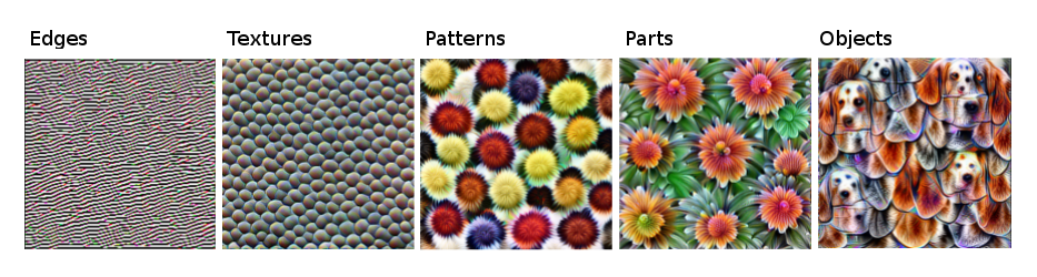
ภาพประกอบ 7.1: Features learned by a convolutional neural network (Inception V1) trained on the ImageNet data. The features range from simple features in the lower convolutional layers (left) to more abstract features in the higher convolutional layers (right). Figure from Olah, et al. 2017 (CC-BY 4.0) https://distill.pub/2017/feature-visualization/appendix/.

• The first convolutional layer(s) learn features such as edges and simple textures.
• Later convolutional layers learn features such as more complex textures and patterns.
• The last convolutional layers learn features such as objects or parts of objects.
• The fully connected layers learn to connect the activations from the high-level features to the individual classes to be predicted.

Cool. But how do we actually get those hallucinatory images?

7.1.1 Feature Visualization

The approach of making the learned features explicit is called Feature Visualization. Feature visualization for a unit of a neural network is done by finding the input that maximizes the activation of that unit.

"Unit" refers either to individual neurons, channels (also called feature maps), entire layers or the final class probability in classification (or the corresponding pre-softmax neuron, which is recommended). Individual neurons are atomic units of the network, so we would get the most information by creating feature visualizations for each neuron. But there is a problem: Neural networks often contain millions of neurons. Looking at each neuron's feature visualization would take too long. The channels (sometimes called activation maps) as units are a good choice for feature visualization. We can go one step further and visualize an entire convolutional layer. Layers as a unit are used for Google's DeepDream, which repeatedly adds the visualized features of a layer to the original image, resulting in a dream-like version of the input.

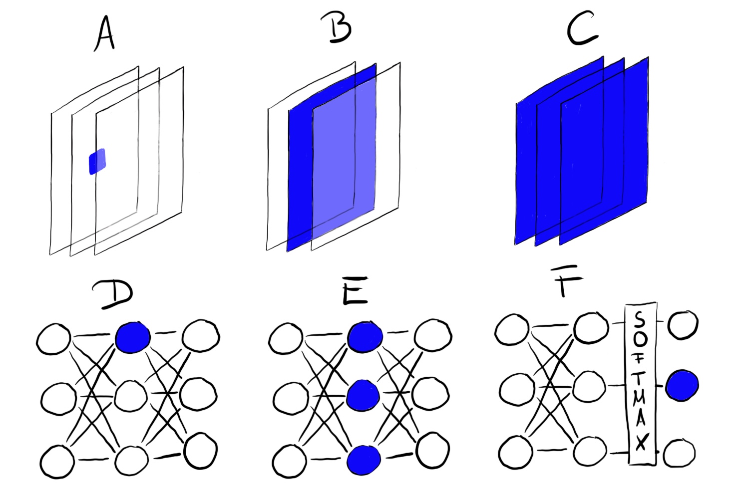
ภาพประกอบ 7.2: Feature visualization can be done for different units. A) Convolution neuron, B) Convolution channel, C) Convolution layer, D) Neuron, E) Hidden layer, F) Class probability neuron (or corresponding pre-softmax neuron)

7.1.1.1 Feature Visualization through Optimization

In mathematical terms, feature visualization is an optimization problem. We assume that the weights of the neural network are fixed, which means that the network is trained. We are looking for a new image that maximizes the (mean) activation of a unit, here a single neuron:

\[img^*=\arg\max_{img}h_{n,x,y,z}(img)\]

The function \(h\) is the activation of a neuron, img the input of the network (an image), x and y describe the spatial position of the neuron, n specifies the layer and z is the channel index. For the mean activation of an entire channel z in layer n we maximize:

\[img^*=\arg\max_{img}\sum_{x,y}h_{n,x,y,z}(img)\]

In this formula, all neurons in channel z are equally weighted. Alternatively, you can also maximize random directions, which means that the neurons would be multiplied by different parameters, including negative directions. In this way, we study how the neurons interact within the channel. Instead of maximizing the activation, you can also minimize the activation (which corresponds to maximizing the negative direction). Interestingly, when you maximize the negative direction you get very different features for the same unit:

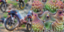
ภาพประกอบ 7.3: Positive (left) and negative (right) activation of Inception V1 neuron 484 from layer mixed4d pre relu. While the neuron is maximally activated by wheels, something which seems to have eyes yields a negative activation. Code: https://colab.research.google.com/github/tensorflow/lucid/blob/master/notebooks/feature-visualization/negative_neurons.ipynb

We can address this optimization problem in different ways. First, why should we generate new images? We could simply search through our training images and select those that maximize the activation. This is a valid approach, but using training data has the problem that elements on the images can be correlated and we can't see what the neural network is really looking for. If images that yield a high activation of a certain channel show a dog and a tennis ball, we don't know whether the neural network looks at the dog, the tennis ball or maybe at both.

The other approach is to generate new images, starting from random noise. To obtain meaningful visualizations, there are usually constraints on the image, e.g. that only small changes are allowed. To reduce noise in the feature visualization, you can apply jittering, rotation or scaling to the image before the optimization step. Other regularization options include frequency penalization (e.g. reduce variance of neighboring pixels) or generating images with learned priors, e.g. with generative adversarial networks (GANs) ⁷⁵ or denoising autoencoders ⁷⁶.

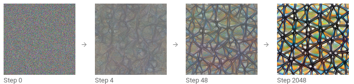
ภาพประกอบ 7.4: Iterative optimization from random image to maximizing activation. Olah, et al. 2017 (CC-BY 4.0) https://distill.pub/2017/feature-visualization/.

If you want to dive a lot deeper into feature visualization, take a look at the distill.pub online journal, especially the feature visualization post by Olah et al. ⁷⁷, from which I used many of the images, and also about the building blocks of interpretability ⁷⁸.

7.1.1.2 Connection to Adversarial Examples

There is a connection between feature visualization and adversarial examples: Both techniques maximize the activation of a neural network unit. For adversarial examples, we look for the maximum activation of the neuron for the adversarial (= incorrect) class. One difference is the image we start with: For adversarial examples, it is the image for which we want to generate the adversarial image. For feature visualization it is, depending on the approach, random noise.

7.1.1.3 Text and Tabular Data

The literature focuses on feature visualization for convolutional neural networks for image recognition. Technically, there is nothing to stop you from finding the input that maximally activates a neuron of a fully connected neural network for tabular data or a recurrent neural network for text data. You might not call it feature visualization any longer, since the "feature" would be a tabular data input or text. For credit default prediction, the inputs might be the number of prior credits, number of mobile contracts, address and dozens of other features. The learned feature of a neuron would then be a certain combination of the dozens of features. For recurrent neural networks, it is a bit nicer to visualize what the network learned: Karpathy et. al (2015)⁷⁹ showed that recurrent neural networks indeed have neurons that learn interpretable features. They trained a character-level model, which predicts the next character in the sequence from the previous characters. Once an opening brace "(" occurred, one of the neurons got highly activated, and got de-activated when the matching closing bracket ")" occurred. Other neurons fired at the end of a line. Some neurons fired in URLs. The difference to the feature visualization for CNNs is that the examples were not found through optimization, but by studying neuron activations in the training data.

Some of the images seem to show well-known concepts like dog snouts or buildings. But how can we be sure? The Network Dissection method links human concepts with individual neural network units. Spoiler alert: Network Dissection requires extra datasets that someone has labeled with human concepts.

7.1.2 Network Dissection

The Network Dissection approach by Bau & Zhou et al. (2017) ⁸⁰ quantifies the interpretability of a unit of a convolutional neural network. It links highly activated areas of CNN channels with human concepts (objects, parts, textures, colors, ...).

The channels of a convolutional neural network learn new features, as we saw in the chapter on Feature Visualization. But these visualizations do not prove that a unit has learned a certain concept. We also do not have a measure for how well a unit detects e.g. sky scrapers. Before we go into the details of Network Dissection, we have to talk about the big hypothesis that is behind that line of research. The hypothesis is: Units of a neural network (like convolutional channels) learn disentangled concepts.

The Question of Disentangled Features

Do (convolutional) neural networks learn disentangled features? Disentangled features mean that individual network units detect specific real world concepts. Convolutional channel 394 might detect sky scrapers, channel 121 dog snouts, channel 12 stripes at 30 degree angle ... The opposite of a disentangled network is a completely entangled network. In a completely entangled network, for example, there would be no individual unit for dog snouts. All channels would contribute to the recognition of dog snouts.

Disentangled features imply that the network is highly interpretable. Let us assume we have a network with completely disentangled units that are labeled with known concepts. This would open up the possibility to track the network's decision making process. For example, we could analyze how the network classifies wolves against huskeys. First, we identify the "huskey"-unit. We can check whether this unit depends on the "dog snout", "fluffy fur" and "snow"-units from the previous layer. If it does, we know that it will misclassify an image of a huskey with a snowy background as a wolf. In a disentangled network, we could identify problematic non-causal correlations. We could automatically list all highly activated units and their concepts to explain an individual prediction. We could easily detect bias in the neural network. For example, did the network learn a "white skin" feature to predict salary?

Spoiler-alert: Convolutional neural networks are not perfectly disentangled. We will now look more closely at Network Dissection to find out how interpretable neural networks are.

7.1.2.1 Network Dissection Algorithm

Network Dissection has three steps:

1. Get images with human-labeled visual concepts, from stripes to skyscrapers.
2. Measure the CNN channel activations for these images.
3. Quantify the alignment of activations and labeled concepts.

The following figure visualizes how an image is forwarded to a channel and matched with the labeled concepts.

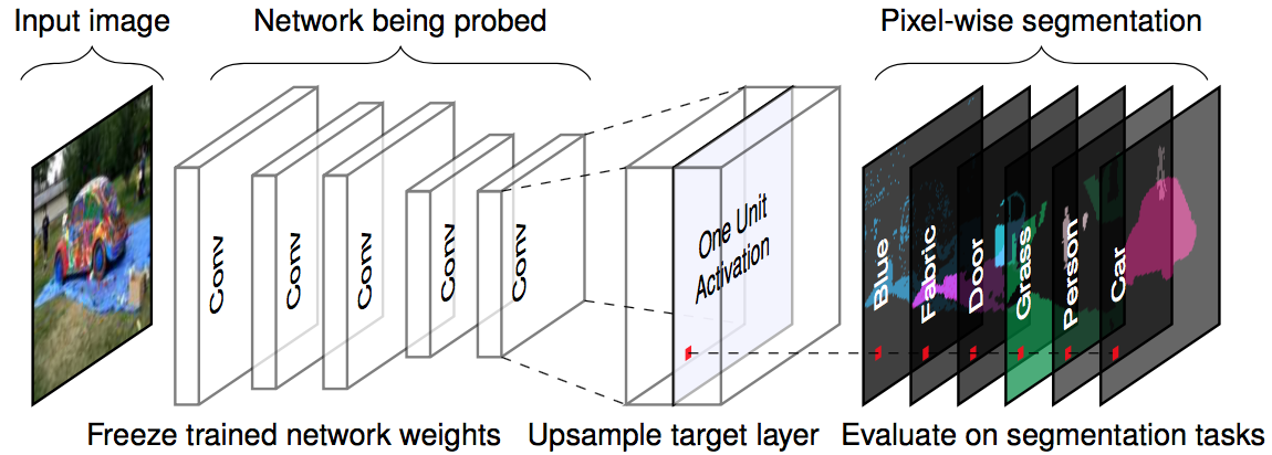
ภาพประกอบ 7.5: For a given input image and a trained network (fixed weights), we forward propagate the image up to the target layer, upscale the activations to match the original image size and compare the maximum activations with the ground truth pixel-wise segmentation. Figure originally from Bau & Zhou et. al (2017).

Step 1: Broden dataset

The first difficult but crucial step is data collection. Network Dissection requires pixel-wise labeled images with concepts of different abstraction levels (from colors to street scenes). Bau & Zhou et. al combined a couple of datasets with pixel-wise concepts. They called this new dataset 'Broden', which stands for broadly and densely labeled data. The Broden dataset is segmented to the pixel level mostly, for some datasets the whole image is labeled. Broden contains 60,000 images with over 1,000 visual concepts in different abstraction levels: 468 scenes, 585 objects, 234 parts, 32 materials, 47 textures and 11 colors. The following figure shows sample images from the Broden dataset.

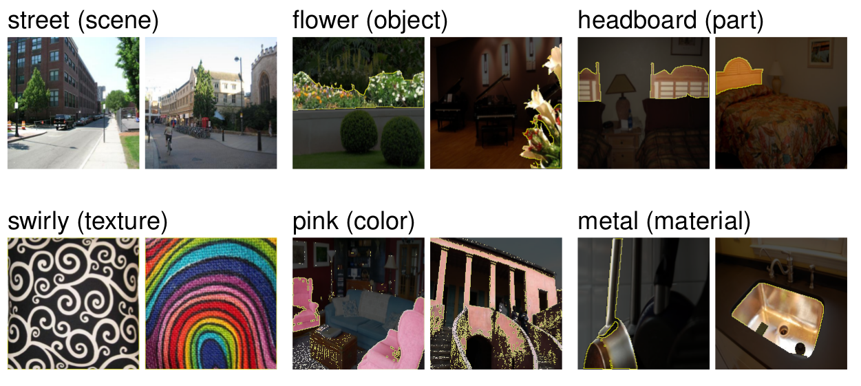
ภาพประกอบ 7.6: Example images from the Broden dataset. Figure originally from Bau & Zhou et. al (2017).

Step 2: Retrieve network activations

Next, we create the masks of the top activated areas per channel and per image. At this point the concept labels are not yet involved.

• For each convolutional channel k:
  • For each image x in the Broden dataset
    • Forward propagate image x to the target layer containing channel k.
    • Extract the pixel activations of convolutional channel k: \(A_k(x)\)
  • Calculate distribution of pixel activations \(\alpha_k\) over all images
  • Determine the 0.005-quantile level \(T_k\) of activations \(\alpha_k\). This means 0.5% of all activations of channel k for image x are greater than \(T_k\).
  • For each image x in the Broden dataset:
    • Scale the (possibly) lower-resolution activation map \(A_k(x)\) to the resolution of image x. We call the result \(S_k(x)\).
    • Binarize the activation map: A pixel is either on or off, depending on whether it exceeds the activation threshold \(T_k\). The new mask is \(M_k(x)=S_k(x)\geq{}T_k(x)\).

Step 3: Activation-concept alignment

After step 2 we have one activation mask per channel and image. These activation masks mark highly activated areas. For each channel we want to find the human concept that activates that channel. We find the concept by comparing the activation masks with all labeled concepts. We quantify the alignment between activation mask k and concept mask c with the Intersection over Union (IoU) score:

\[IoU_{k,c}=\frac{\sum|M_k(x)\bigcap{}L_c(x)|}{\sum|M_k(x)\bigcup{}L_c(x)|}\]

where \(|\cdot|\) is the cardinality of a set. Intersection over union compares the alignment between two areas. \(IoU_{k,c}\) can be interpreted as the accuracy with which unit k detects concept c. We call unit k a detector of concept c when \(IoU_{k,c}>0.04\). This threshold was chosen by Bau & Zhou et. al.

The following figure illustrates intersection and union of activation mask and concept mask for a single image:

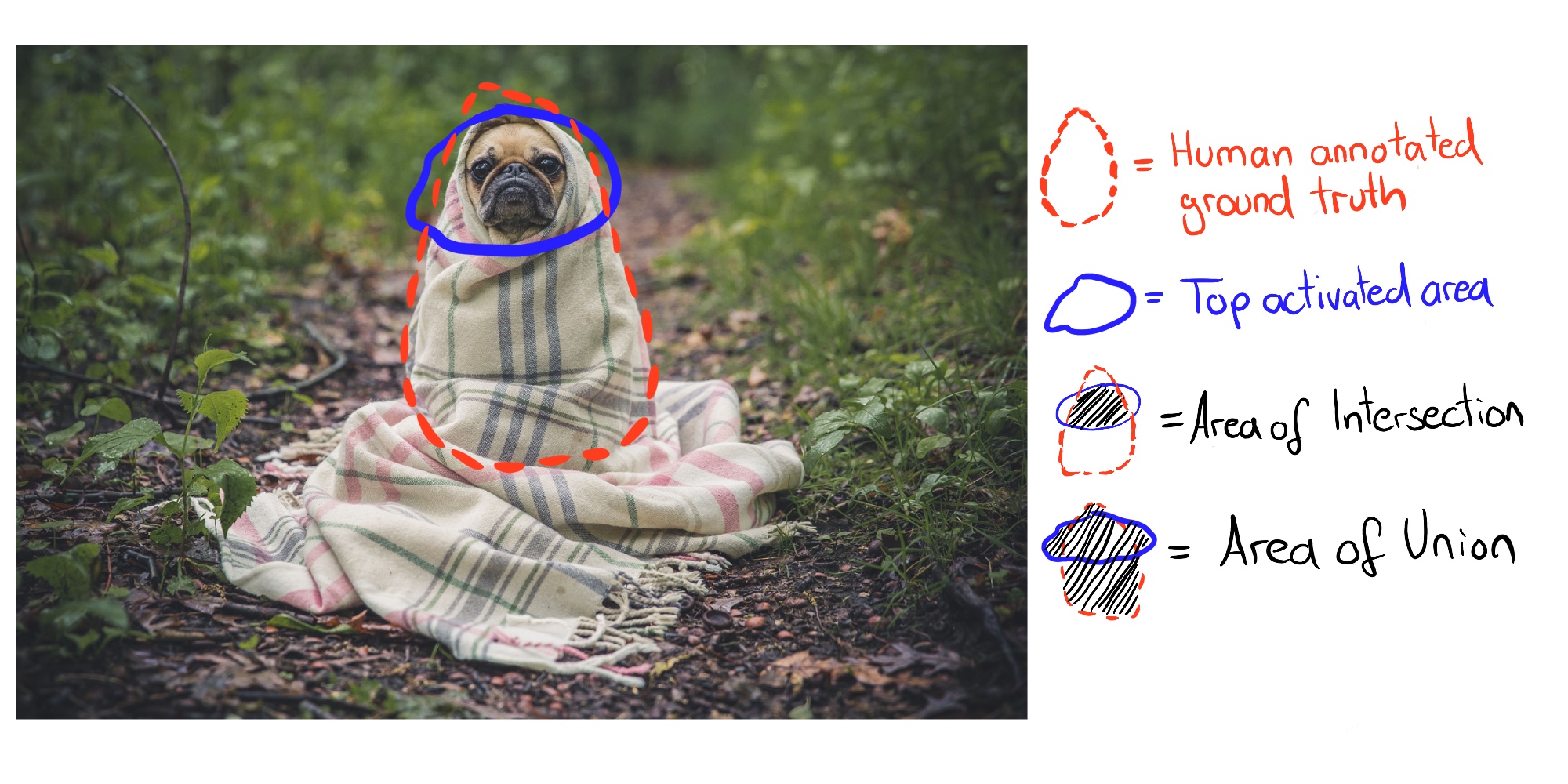
ภาพประกอบ 7.7: The Intersection over Union (IoU) is computed by comparing the human ground truth annotation and the top activated pixels.

The following figure shows a unit that detects dogs:

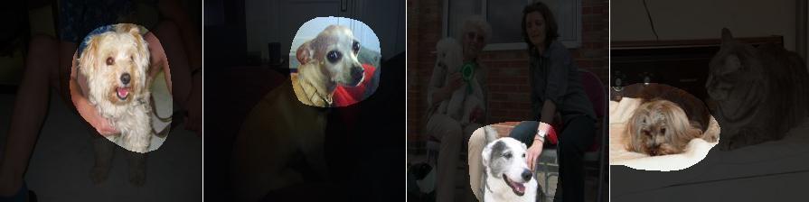
ภาพประกอบ 7.8: Activation mask for inception_4e channel 750 which detects dogs with \(IoU=0.203\). Figure originally from Bau & Zhou et. al (2017).

7.1.2.2 Experiments

The Network Dissection authors trained different network architectures (AlexNet, VGG, GoogleNet, ResNet) from scratch on different datasets (ImageNet, Places205, Places365). ImageNet contains 1.6 million images from 1000 classes that focus on objects. Places205 and Places365 contain 2.4 million / 1.6 million images from 205 / 365 different scenes. They additionally trained AlexNet on self-supervised training tasks such as predicting video frame order or colorizing images. For many of these different settings, they counted the number of unique concept detectors as a measure of interpretability. Here are some of the findings:

• The networks detect lower-level concepts (colors, textures) at lower layers and higher-level concepts (parts, objects) at higher layers. We have already seen this in the Feature Visualizations.
• Batch normalization reduces the number of unique concept detectors.
• Many units detect the same concept. For example, there are 95 (!) dog channels in VGG trained on ImageNet when using \(IoU \geq 0.04\) as detection cutoff (4 in conv4_3, 91 in conv5_3, see project website).
• Increasing the number of channels in a layer increases the number of interpretable units.
• Random initializations (training with different random seeds) result in slightly different numbers of interpretable units.
• ResNet is the network architecture with the largest number of unique detectors, followed by VGG, GoogleNet and AlexNet last.
• The largest number of unique concept detectors are learned for Places356, followed by Places205 and ImageNet last.
• The number of unique concept detectors increases with the number of training iterations.
  

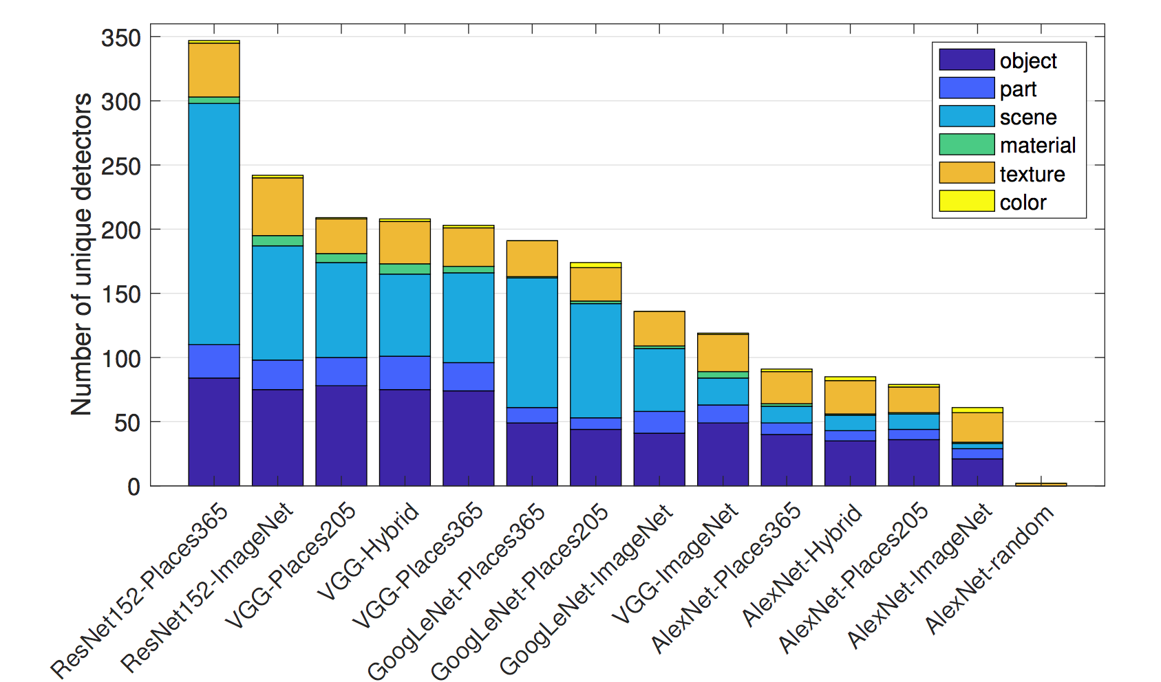
  ภาพประกอบ 7.9: ResNet trained on Places365 has the highest number of unique detectors. AlexNet with random weights has the lowest number of unique detectors and serves as baseline. Figure originally from Bau & Zhou et. al (2017).

• Networks trained on self-supervised tasks have fewer unique detectors compared to networks trained on supervised tasks.
• In transfer learning, the concept of a channel can change. For example, a dog detector became a waterfall detector. This happened in a model that was initially trained to classify objects and then fine-tuned to classify scenes.
• In one of the experiments, the authors projected the channels onto a new rotated basis. This was done for the VGG network trained on ImageNet. "Rotated" does not mean that the image was rotated. "Rotated" means that we take the 256 channels from the conv5 layer and compute new 256 channels as linear combinations of the original channels. In the process, the channels get entangled. Rotation reduces interpretability, i.e., the number of channels aligned with a concept decreases. The rotation was designed to keep the performance of the model the same. The first conclusion: Interpretability of CNNs is axis-dependent. This means that random combinations of channels are less likely to detect unique concepts. The second conclusion: Interpretability is independent of discriminative power. The channels can be transformed with orthogonal transformations while the discriminative power remains the same, but interpretability decreases.
  

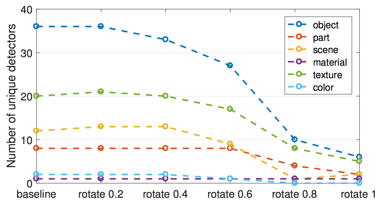
  ภาพประกอบ 7.10: The number of unique concept detectors decreases when the 256 channels of AlexNet conv5 (trained on ImageNet) are gradually changed to a basis using a random orthogonal transformation. Figure originally from Bau & Zhou et. al (2017).

The authors also used Network Dissection for Generative Adversarial Networks (GANs). You can find Network Dissection for GANs on the project's website.

7.1.3 Advantages

Feature visualizations give unique insight into the working of neural networks, especially for image recognition. Given the complexity and opacity of neural networks, feature visualization is an important step in analyzing and describing neural networks. Through feature visualization, we have learned that neural networks first learn simple edge and texture detectors and more abstract part and object detectors in higher layers. Network dissection expands those insights and makes interpretability of network units measurable.

Network dissection allows us to automatically link units to concepts, which is very convenient.

Feature visualization is a great tool to communicate in a non-technical way how neural networks work.

With network dissection, we can also detect concepts beyond the classes in the classification task. But we need datasets that contain images with pixel-wise labeled concepts.

Feature visualization can be combined with feature attribution methods, which explain which pixels were important for the classification. The combination of both methods allows to explain an individual classification along with local visualization of the learned features that were involved in the classification. See The Building Blocks of Interpretability from distill.pub.

Finally, feature visualizations make great desktop wallpapers and T-Shirts prints.

7.1.4 Disadvantages

Many feature visualization images are not interpretable at all, but contain some abstract features for which we have no words or mental concept. The display of feature visualizations along with training data can help. The images still might not reveal what the neural network reacted to and only show something like "maybe there has to be something yellow in the images". Even with Network Dissection some channels are not linked to a human concept. For example, layer conv5_3 from VGG trained on ImageNet has 193 channels (out of 512) that could not be matched with a human concept.

There are too many units to look at, even when "only" visualizing the channel activations. For Inception V1 there are already over 5000 channels from 9 convolutional layers. If you also want to show the negative activations plus a few images from the training data that maximally or minimally activate the channel (let's say 4 positive, 4 negative images), then you must already display more than 50 000 images. At least we know -- thanks to Network Dissection -- that we do not need to investigate random directions.

Illusion of Interpretability? The feature visualizations can convey the illusion that we understand what the neural network is doing. But do we really understand what is going on in the neural network? Even if we look at hundreds or thousands of feature visualizations, we cannot understand the neural network. The channels interact in a complex way, positive and negative activations are unrelated, multiple neurons might learn very similar features and for many of the features we do not have equivalent human concepts. We must not fall into the trap of believing we fully understand neural networks just because we believe we saw that neuron 349 in layer 7 is activated by daisies. Network Dissection showed that architectures like ResNet or Inception have units that react to certain concepts. But the IoU is not that great and often many units respond to the same concept and some to no concept at all. They channels are not completely disentangled and we cannot interpret them in isolation.

For Network Dissection, you need datasets that are labeled on the pixel level with the concepts. These datasets take a lot of effort to collect, since each pixel needs to be labeled, which usually works by drawing segments around objects on the image.

Network Dissection only aligns human concepts with positive activations but not with negative activations of channels. As the feature visualizations showed, negative activations seem to be linked to concepts. This might be fixed by additionally looking at the lower quantile of activations.

7.1.5 Software and Further Material

There is an open-source implementation of feature visualization called Lucid. You can conveniently try it in your browser by using the notebook links that are provided on the Lucid Github page. No additional software is required. Other implementations are tf_cnnvis for TensorFlow, Keras Filters for Keras and DeepVis for Caffe.

Network Dissection has a great project website. Next to the publication, the website hosts additional material such as code, data and visualizations of activation masks.

---

75. Nguyen, Anh, et al. "Synthesizing the preferred inputs for neurons in neural networks via deep generator networks." Advances in Neural Information Processing Systems. 2016.↩

76. Nguyen, Anh, et al. "Plug & play generative networks: Conditional iterative generation of images in latent space." Proceedings of the IEEE Conference on Computer Vision and Pattern Recognition. 2017.↩

77. Olah, et al., "Feature Visualization", Distill, 2017.↩

78. Olah, et al., "The Building Blocks of Interpretability", Distill, 2018.↩

79. Karpathy, Andrej, Justin Johnson, and Li Fei-Fei. "Visualizing and understanding recurrent networks." arXiv preprint arXiv:1506.02078 (2015).↩

80. Bau, David, et al. "Network dissection: Quantifying interpretability of deep visual representations." Proceedings of the IEEE Conference on Computer Vision and Pattern Recognition. 2017.↩