7.3 Detecting Concepts

Author: Fangzhou Li @ University of California, Davis

This chapter is currently only available in this web version. ebook and print will follow.

So far, we have encountered many methods to explain black-box models through feature attribution. However, there are some limitations regarding the feature-based approach. First, features are not necessarily user-friendly in terms of interpretability. For example, the importance of a single pixel in an image usually does not convey much meaningful interpretation. Second, the expressiveness of a feature-based explanation is constrained by the number of features.

The concept-based approach addresses both limitations mentioned above. A concept can be any abstraction, such as a color, an object, or even an idea. Given any user-defined concept, although a neural network might not be explicitly trained with the given concept, the concept-based approach detects that concept embedded within the latent space learned by the network. In other words, the concept-based approach can generate explanations that are not limited by the feature space of a neural network.

In this chapter, we will primarily focus on the Testing with Concept Activation Vectors (TCAV) paper by Kim et al.⁹⁰

7.3.1 TCAV: Testing with Concept Activation Vectors

TCAV is proposed to generate global explanations for neural networks. For any given concept, TCAV measures the extent of that concept's influence on the model's prediction for a certain class. For example, TCAV can answer questions such as how the concept of "striped" influences a model classifying an image as a "zebra". Since TCAV describes the relationship between a concept and a class, instead of explaining a single prediction, it provides useful global interpretation for a model's overall behavior.

7.3.1.1 Concept Activation Vector (CAV)

A CAV is simply the numerical representation that generalizes a concept in the activation space of a neural network layer. A CAV, denoted as \(v_l^C\), depends on a concept \(C\) and a neural network layer \(l\), where \(l\) is also called as a bottleneck of the model. For calculating the CAV of a concept \(C\), first, we need to prepare two datasets: a concept dataset which represents \(C\) and a random dataset that consists of arbitrary data. For instance, to define the concept of "striped", we can collect images of striped objects as the concept dataset, while the random dataset is a group of random images without stripes. Next, we target a hidden layer \(l\) and train a binary classifier which separates the activations generated by the concept set from those generated by the random set. The coefficient vector of this trained binary classifier is then the CAV \(v_l^C\). In practice, we can use a SVM or a logistic regression model as the binary classifier. Lastly, given an image input \(x\), we can measure its "conceptual sensitivity" by calculating the directional derivative of the prediction in the direction of the unit CAV:

\[S_{C,k,l}(x)=\nabla h_{l,k}(f_l(x))\cdot v_l^C\]

where \(f_l\) maps the input \(x\) to the activation vector of the layer \(l\) and \(h_{l,k}\) maps the activation vector to the logit output of class \(k\).

Mathematically, the sign of \(x\)'s conceptual sensitivity only depends on the angle between the gradient of \(h_{l,k}(f_l(x))\) and \(v_l^C\). If the angle is greater than 90 degrees, \(S_{C,k,l}(x)\) will be positive, and if the angle is less than 90 degrees, \(S_{C,k,l}(x)\) will be negative. Since the gradient \(\nabla h_{l,k}\) points to the direction that maximizes the output the most rapidly, conceptual sensitivity, intuitively, indicates whether \(v_l^C\) points to the similar direction that maximizes \(h_{l,k}\). Thus, \(S_{C,k,l}(x)>0\) can be interpreted as concept \(C\) encouraging the model to classify \(x\) into class \(k\).

7.3.1.2 Testing with CAVs (TCAV)

In the last paragraph, we have learned how to calculate the conceptual sensitivity of a single data point. However, our goal is to produce a global explanation that indicates an overall conceptual sensitivity of an entire class. A very straightforward approach done by TCAV is to calculate the ratio of inputs with positive conceptual sensitivities to the number of inputs for a class:

\[TCAV_{Q_{C,k,l}}=\frac{|{x\in X_k:S_{C,k,l}(x)>0}|}{|X_k|}\]

Going back to our example, we are interested in how the concept of "striped" influences the model while classifying images as "zebra". We collect data that are labeled as "zebra" and calculate conceptual sensitivity for each input image. Then the TCAV score of the concept "striped" with predicting class "zebra" is the number of "zebra" images that have positive conceptual sensitivities divided by the total number of the "zebra" images. In other words, a \(TCAV_{Q_{"striped","zebra",l}}\) equal to 0.8 indicates that 80% of predictions for "zebra" class are positively influenced by the concept of "striped".

This looks great, but how do we know our TCAV score is meaningful? After all, a CAV is trained by user-selected concept and random datasets. If datasets used to train the CAV are bad, the explanation can be misleading and useless. And thus, we perform a simple statistical significance test to help TCAV become more reliable. That is, instead of training only one CAV, we train multiple CAVs using different random datasets. A meaningful concept should generate CAVs with consistent TCAV scores. More detailed test procedure is shown as the following:

1. Collect \(N\) random datasets, where it is recommended that \(N\) is at least 10.
2. Fix the concept dataset and calculate TCAV score using each of \(N\) random datasets.
3. Apply a two-sided t-test to \(N\) TCAV scores against another \(N\) TCAV scores generated by a random CAV. A random CAV can be obtained by choosing a random dataset as the concept dataset.

It is also suggested to apply a multiple testing correction method here if you have multiple hypotheses. The original paper uses Bonferroni correction, and here the number of hypotheses is equal to the number of concepts you are testing.

7.3.2 Example

Let us see an example available on the TCAV GitHub. Continuing the “zebra” class example we have been using previously, this example shows the result of the TCAV scores of “striped”, “zigzagged”, and “dotted” concepts. The image classifier we are using is InceptionV3⁹¹, a convolutional neural network trained using ImageNet data. Each concept or random dataset contains 50 images, and we are using 10 random datasets for the statistical significance test with the significance level of 0.05. We are not using the Bonferroni correction because we only have a few random datasets, but it is recommended to add the correction in practice to avoid false discovery.

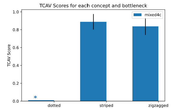
ภาพประกอบ 7.11: The example of measuring TCAV scores of three concepts for the model predicting “zebra”. The targeted bottleneck is a layer called “mixed4c”. A star sign above “dotted” indicates that “dotted” has not passed the statistical significance test, i.e., having the p-value larger than 0.05. Both “striped” and “zigzagged” have passed the test, and both concepts are useful for the model to identify “zebra” images according to TCAV. Figure originally from the TCAV GitHub.

In practice, you may want to use more than 50 images in each dataset to train better CAVs. You may also want to use more than 10 random datasets to perform better statistical significance tests. You can also apply TCAV to multiple bottlenecks to have a more thorough observation.

7.3.3 Advantages

Since users are only required to collect data for training the concepts that they are interested in, TCAV does not require users to have machine learning expertise. This allows TCAV to be extremely useful for domain experts to evaluate their complicated neural network models.

Another unique characteristic of TCAV is its customizability enabled by TCAV's explanations beyond feature attribution. Users can investigate any concept as long as the concept can be defined by its concept dataset. In other words, a user can control the balance between the complexity and the interpretability of explanations based on their needs: If a domain expert understands the problem and concept very well, they can shape the concept dataset using more complicated data to generate a more fine-grained explanation.

Finally, TCAV generates global explanations that relate concepts to any class. A global explanation gives you an idea that whether your overall model behaves properly or not, which usually cannot be done by local explanations. And thus, TCAV can be used to identify potential "flaws" or "blind spots" happened during the model training: Maybe your model has learned to weight a concept inappropriately. If a user can identify those ill-learned concepts, one can use the knowledge to improve their model. Let us say there is a classifier that predicts "zebra" with a high accuracy. TCAV, however, shows that the classifier is more sensitive towards the concept of "dotted" instead of "striped". This might indicate that the classifier is accidentally trained by an unbalanced dataset, allowing you to improve the model by either adding more "striped zebra" images or less "dotted zebra" images to the training dataset.

7.3.4 Disadvantages

TCAV might perform badly on shallower neural networks. As many papers suggested ⁹², concepts in deeper layers are more separable. If a network is too shallow, its layers may not be capable of separating concepts clearly so that TCAV is not applicable.

Since TCAV requires additional annotations for concept datasets, it can be very expensive for tasks that do not have ready labelled data.

Although TCAV is hailed because of its customizability, it is difficult to apply to concepts that are too abstract or general. This is mainly because TCAV describes a concept by its corresponding concept dataset. The more abstract or general a concept is, such as "happiness", the more data are required to train a CAV for that concept.

Though TCAV gains popularity in applying to image data, it has relatively limited applications in text data and tabular data.

7.3.5 Bonus: Other Concept-based Approaches

The concept-based approach has attracted increasing popularity in recent, and there are many new methods inspired by the utilization of concepts. Here we would like to briefly mention these methods, and we recommend you read the original works if you are interested.

Automated Concept-based Explanation (ACE)⁹³ can be seen as the automated version of TCAV. ACE goes through a set of images of a class and automatically generates concepts based on the clustering of image segments.

Concept bottleneck models (CBM)⁹⁴ are intrinsically interpretable neural networks. A CBM is similar to an encoder-decoder model, where the first half of the CBM maps inputs to concepts, and the second half uses the mapped concepts to predict model outputs. Each neuron activation of the bottleneck layer then represents the importance of a concept. Furthermore, users can do intervention to the neuron activations of the bottleneck to generate counterfactual explanations of the model.

Concept whitening (CW)⁹⁵ is another approach to generate intrinsically interpretable image classifiers. To use CW, one just simply substitutes a normalization layer, such as a batch normalization layer, with a CW layer. And thus, CW is very useful when users want to transform their pre-trained image classifiers to be intrinsically interpretable, while maintaining the model performance. CW is heavily inspired by whitening transformation, and we highly recommend you to study the mathematics behind whitening transformation if you are interested in learning more about CW.

7.3.6 Software

The official Python library of TCAV requires Tensorflow, but there are other versions implemented online. The easy-to-use Jupyter notebooks are also accessible on the tensorflow/tcav.

---

90. Kim, Been, et al. "Interpretability beyond feature attribution: Quantitative testing with concept activation vectors (tcav)." Proceedings of the 35th International Conference on Machine Learning (2018).↩

91. Szegedy, Christian, et al. "Rethinking the Inception architecture for computer vision." Proceedings of the IEEE conference on computer vision and pattern recognition, 2818-2826 (2016).↩

92. Alain, Guillaume, et al. "Understanding intermediate layers using linear classifier probes." arXiv preprint arXiv:1610.01644 (2018).↩

93. Ghorbani, Amirata, et al. "Towards automatic concept-based explanations." Advances in Neural Information Processing Systems 32 (2019).↩

94. Koh, Pang Wei, et al. "Concept bottleneck models." Proceedings of the 37th International Conference on Machine Learning (2020).↩

95. Chen, Zhi, et al. "Concept Whitening for Interpretable Image Recognition." Nature Machine Intelligence 2, 772–782 (2020).↩