4.1 Linear Regression
A linear regression model predicts the target as a weighted sum of the feature inputs. The linearity of the learned relationship makes the interpretation easy. Linear regression models have long been used by statisticians, computer scientists and other people who tackle quantitative problems.
Linear models can be used to model the dependence of a regression target y on some features x. The learned relationships are linear and can be written for a single instance i as follows:
\[y=\beta_{0}+\beta_{1}x_{1}+\ldots+\beta_{p}x_{p}+\epsilon\]
The predicted outcome of an instance is a weighted sum of its p features. The betas (\(\beta_{j}\)) represent the learned feature weights or coefficients. The first weight in the sum (\(\beta_0\)) is called the intercept and is not multiplied with a feature. The epsilon (\(\epsilon\)) is the error we still make, i.e. the difference between the prediction and the actual outcome. These errors are assumed to follow a Gaussian distribution, which means that we make errors in both negative and positive directions and make many small errors and few large errors.
Various methods can be used to estimate the optimal weight. The ordinary least squares method is usually used to find the weights that minimize the squared differences between the actual and the estimated outcomes:
\[\hat{\boldsymbol{\beta}}=\arg\!\min_{\beta_0,\ldots,\beta_p}\sum_{i=1}^n\left(y^{(i)}-\left(\beta_0+\sum_{j=1}^p\beta_jx^{(i)}_{j}\right)\right)^{2}\]
We will not discuss in detail how the optimal weights can be found, but if you are interested, you can read chapter 3.2 of the book "The Elements of Statistical Learning" (Friedman, Hastie and Tibshirani 2009)16 or one of the other online resources on linear regression models.
The biggest advantage of linear regression models is linearity: It makes the estimation procedure simple and, most importantly, these linear equations have an easy to understand interpretation on a modular level (i.e. the weights). This is one of the main reasons why the linear model and all similar models are so widespread in academic fields such as medicine, sociology, psychology, and many other quantitative research fields. For example, in the medical field, it is not only important to predict the clinical outcome of a patient, but also to quantify the influence of the drug and at the same time take sex, age, and other features into account in an interpretable way.
Estimated weights come with confidence intervals. A confidence interval is a range for the weight estimate that covers the "true" weight with a certain confidence. For example, a 95% confidence interval for a weight of 2 could range from 1 to 3. The interpretation of this interval would be: If we repeated the estimation 100 times with newly sampled data, the confidence interval would include the true weight in 95 out of 100 cases, given that the linear regression model is the correct model for the data.
Whether the model is the "correct" model depends on whether the relationships in the data meet certain assumptions, which are linearity, normality, homoscedasticity, independence, fixed features, and absence of multicollinearity.
Linearity
The linear regression model forces the prediction to be a linear combination of features, which is both its greatest strength and its greatest limitation. Linearity leads to interpretable models. Linear effects are easy to quantify and describe. They are additive, so it is easy to separate the effects. If you suspect feature interactions or a nonlinear association of a feature with the target value, you can add interaction terms or use regression splines.
Normality
It is assumed that the target outcome given the features follows a normal distribution. If this assumption is violated, the estimated confidence intervals of the feature weights are invalid.
Homoscedasticity (constant variance)
The variance of the error terms is assumed to be constant over the entire feature space. Suppose you want to predict the value of a house given the living area in square meters. You estimate a linear model that assumes that, regardless of the size of the house, the error around the predicted response has the same variance. This assumption is often violated in reality. In the house example, it is plausible that the variance of error terms around the predicted price is higher for larger houses, since prices are higher and there is more room for price fluctuations. Suppose the average error (difference between predicted and actual price) in your linear regression model is 50,000 Euros. If you assume homoscedasticity, you assume that the average error of 50,000 is the same for houses that cost 1 million and for houses that cost only 40,000. This is unreasonable because it would mean that we can expect negative house prices.
Independence
It is assumed that each instance is independent of any other instance. If you perform repeated measurements, such as multiple blood tests per patient, the data points are not independent. For dependent data you need special linear regression models, such as mixed effect models or GEEs. If you use the "normal" linear regression model, you might draw wrong conclusions from the model.
Fixed features
The input features are considered "fixed". Fixed means that they are treated as "given constants" and not as statistical variables. This implies that they are free of measurement errors. This is a rather unrealistic assumption. Without that assumption, however, you would have to fit very complex measurement error models that account for the measurement errors of your input features. And usually you do not want to do that.
Absence of multicollinearity
You do not want strongly correlated features, because this messes up the estimation of the weights. In a situation where two features are strongly correlated, it becomes problematic to estimate the weights because the feature effects are additive and it becomes indeterminable to which of the correlated features to attribute the effects.
4.1.1 Interpretation
The interpretation of a weight in the linear regression model depends on the type of the corresponding feature.
- Numerical feature: Increasing the numerical feature by one unit changes the estimated outcome by its weight. An example of a numerical feature is the size of a house.
- Binary feature: A feature that takes one of two possible values for each instance. An example is the feature "House comes with a garden". One of the values counts as the reference category (in some programming languages encoded with 0), such as "No garden". Changing the feature from the reference category to the other category changes the estimated outcome by the feature's weight.
- Categorical feature with multiple categories: A feature with a fixed number of possible values. An example is the feature "floor type", with possible categories "carpet", "laminate" and "parquet". A solution to deal with many categories is the one-hot-encoding, meaning that each category has its own binary column. For a categorical feature with L categories, you only need L-1 columns, because the L-th column would have redundant information (e.g. when columns 1 to L-1 all have value 0 for one instance, we know that the categorical feature of this instance takes on category L). The interpretation for each category is then the same as the interpretation for binary features. Some languages, such as R, allow you to encode categorical features in various ways, as described later in this chapter.
- Intercept \(\beta_0\): The intercept is the feature weight for the "constant feature", which is always 1 for all instances. Most software packages automatically add this "1"-feature to estimate the intercept. The interpretation is: For an instance with all numerical feature values at zero and the categorical feature values at the reference categories, the model prediction is the intercept weight. The interpretation of the intercept is usually not relevant because instances with all features values at zero often make no sense. The interpretation is only meaningful when the features have been standardised (mean of zero, standard deviation of one). Then the intercept reflects the predicted outcome of an instance where all features are at their mean value.
The interpretation of the features in the linear regression model can be automated by using following text templates.
Interpretation of a Numerical Feature
An increase of feature \(x_{k}\) by one unit increases the prediction for y by \(\beta_k\) units when all other feature values remain fixed.
Interpretation of a Categorical Feature
Changing feature \(x_{k}\) from the reference category to the other category increases the prediction for y by \(\beta_{k}\) when all other features remain fixed.
Another important measurement for interpreting linear models is the R-squared measurement. R-squared tells you how much of the total variance of your target outcome is explained by the model. The higher R-squared, the better your model explains the data. The formula for calculating R-squared is:
\[R^2=1-SSE/SST\]
SSE is the squared sum of the error terms:
\[SSE=\sum_{i=1}^n(y^{(i)}-\hat{y}^{(i)})^2\]
SST is the squared sum of the data variance:
\[SST=\sum_{i=1}^n(y^{(i)}-\bar{y})^2\]
The SSE tells you how much variance remains after fitting the linear model, which is measured by the squared differences between the predicted and actual target values. SST is the total variance of the target outcome. R-squared tells you how much of your variance can be explained by the linear model. R-squared ranges between 0 for models where the model does not explain the data at all and 1 for models that explain all of the variance in your data.
There is a catch, because R-squared increases with the number of features in the model, even if they do not contain any information about the target value at all. Therefore, it is better to use the adjusted R-squared, which accounts for the number of features used in the model. Its calculation is:
\[\bar{R}^2=1-(1-R^2)\frac{n-1}{n-p-1}\]
where p is the number of features and n the number of instances.
It is not meaningful to interpret a model with very low (adjusted) R-squared, because such a model basically does not explain much of the variance. Any interpretation of the weights would not be meaningful.
Feature Importance
The importance of a feature in a linear regression model can be measured by the absolute value of its t-statistic. The t-statistic is the estimated weight scaled with its standard error.
\[t_{\hat{\beta}_j}=\frac{\hat{\beta}_j}{SE(\hat{\beta}_j)}\]
Let us examine what this formula tells us: The importance of a feature increases with increasing weight. This makes sense. The more variance the estimated weight has (= the less certain we are about the correct value), the less important the feature is. This also makes sense.
4.1.2 Example
In this example, we use the linear regression model to predict the number of rented bikes on a particular day, given weather and calendar information. For the interpretation, we examine the estimated regression weights. The features consist of numerical and categorical features. For each feature, the table shows the estimated weight, the standard error of the estimate (SE), and the absolute value of the t-statistic (|t|).
| Weight | SE | |t| | |
|---|---|---|---|
| (Intercept) | 2399.4 | 238.3 | 10.1 |
| seasonSUMMER | 899.3 | 122.3 | 7.4 |
| seasonFALL | 138.2 | 161.7 | 0.9 |
| seasonWINTER | 425.6 | 110.8 | 3.8 |
| holidayHOLIDAY | -686.1 | 203.3 | 3.4 |
| workingdayWORKING DAY | 124.9 | 73.3 | 1.7 |
| weathersitMISTY | -379.4 | 87.6 | 4.3 |
| weathersitRAIN/SNOW/STORM | -1901.5 | 223.6 | 8.5 |
| temp | 110.7 | 7.0 | 15.7 |
| hum | -17.4 | 3.2 | 5.5 |
| windspeed | -42.5 | 6.9 | 6.2 |
| days_since_2011 | 4.9 | 0.2 | 28.5 |
Interpretation of a numerical feature (temperature): An increase of the temperature by 1 degree Celsius increases the predicted number of bicycles by 110.7, when all other features remain fixed.
Interpretation of a categorical feature ("weathersit"): The estimated number of bicycles is -1901.5 lower when it is raining, snowing or stormy, compared to good weather -- again assuming that all other features do not change. When the weather is misty, the predicted number of bicycles is -379.4 lower compared to good weather, given all other features remain the same.
All the interpretations always come with the footnote that "all other features remain the same". This is because of the nature of linear regression models. The predicted target is a linear combination of the weighted features. The estimated linear equation is a hyperplane in the feature/target space (a simple line in the case of a single feature). The weights specify the slope (gradient) of the hyperplane in each direction. The good side is that the additivity isolates the interpretation of an individual feature effect from all other features. That is possible because all the feature effects (= weight times feature value) in the equation are combined with a plus. On the bad side of things, the interpretation ignores the joint distribution of the features. Increasing one feature, but not changing another, can lead to unrealistic or at least unlikely data points. For example increasing the number of rooms might be unrealistic without also increasing the size of a house.
4.1.3 Visual Interpretation
Various visualizations make the linear regression model easy and quick to grasp for humans.
4.1.3.1 Weight Plot
The information of the weight table (weight and variance estimates) can be visualized in a weight plot. The following plot shows the results from the previous linear regression model.
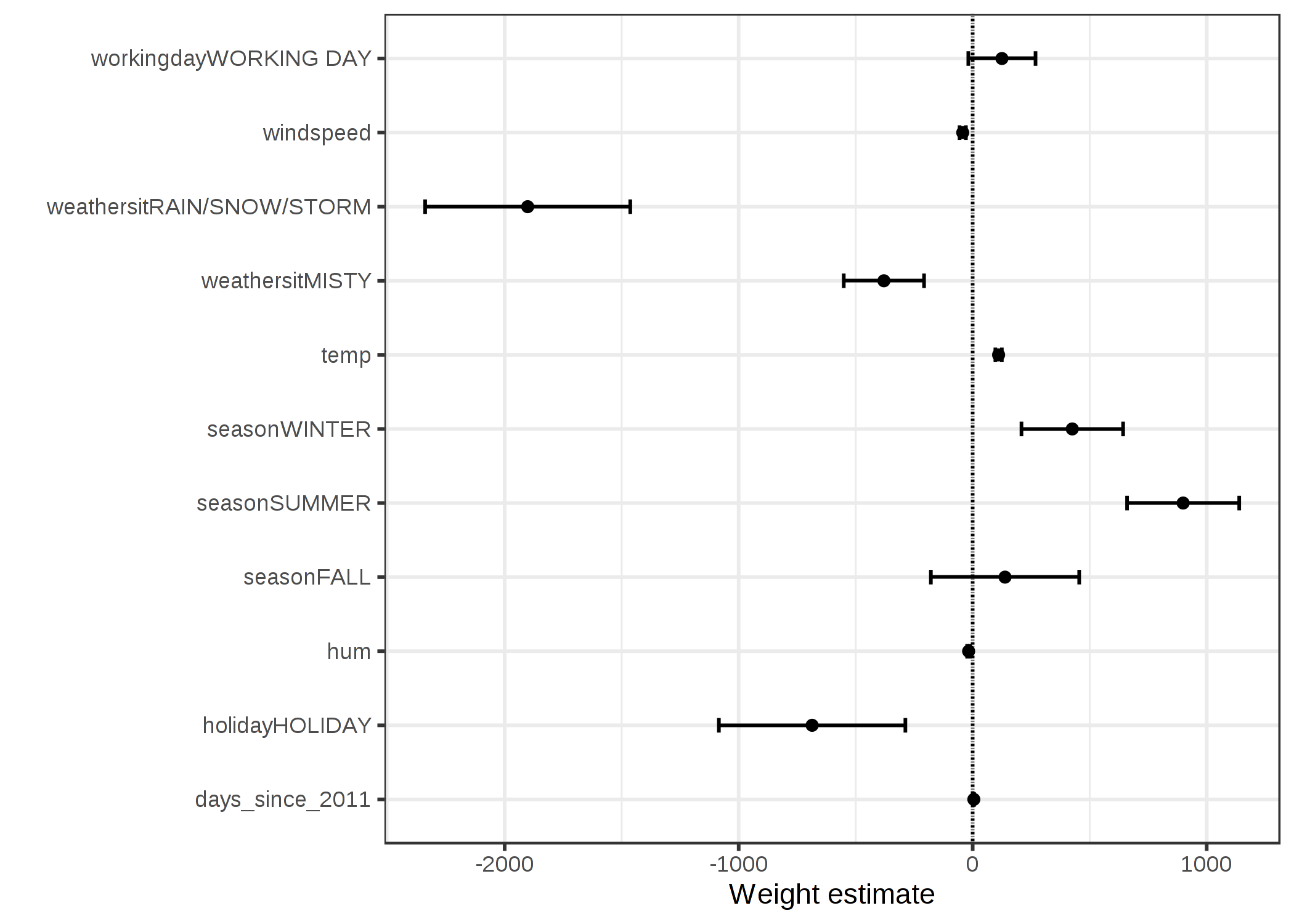
ภาพประกอบ 4.1: Weights are displayed as points and the 95% confidence intervals as lines.
The weight plot shows that rainy/snowy/stormy weather has a strong negative effect on the predicted number of bikes. The weight of the working day feature is close to zero and zero is included in the 95% interval, which means that the effect is not statistically significant. Some confidence intervals are very short and the estimates are close to zero, yet the feature effects were statistically significant. Temperature is one such candidate. The problem with the weight plot is that the features are measured on different scales. While for the weather the estimated weight reflects the difference between good and rainy/stormy/snowy weather, for temperature it only reflects an increase of 1 degree Celsius. You can make the estimated weights more comparable by scaling the features (zero mean and standard deviation of one) before fitting the linear model.
4.1.3.2 Effect Plot
The weights of the linear regression model can be more meaningfully analyzed when they are multiplied by the actual feature values. The weights depend on the scale of the features and will be different if you have a feature that measures e.g. a person's height and you switch from meter to centimeter. The weight will change, but the actual effects in your data will not. It is also important to know the distribution of your feature in the data, because if you have a very low variance, it means that almost all instances have similar contribution from this feature. The effect plot can help you understand how much the combination of weight and feature contributes to the predictions in your data. Start by calculating the effects, which is the weight per feature times the feature value of an instance:
\[\text{effect}_{j}^{(i)}=w_{j}x_{j}^{(i)}\]
The effects can be visualized with boxplots. A box in a boxplot contains the effect range for half of your data (25% to 75% effect quantiles). The vertical line in the box is the median effect, i.e. 50% of the instances have a lower and the other half a higher effect on the prediction. The horizontal lines extend to \(\pm1.5\text{IQR}/\sqrt{n}\), with IQR being the inter quartile range (75% quantile minus 25% quantile). The dots are outliers. The categorical feature effects can be summarized in a single boxplot, compared to the weight plot, where each category has its own row.
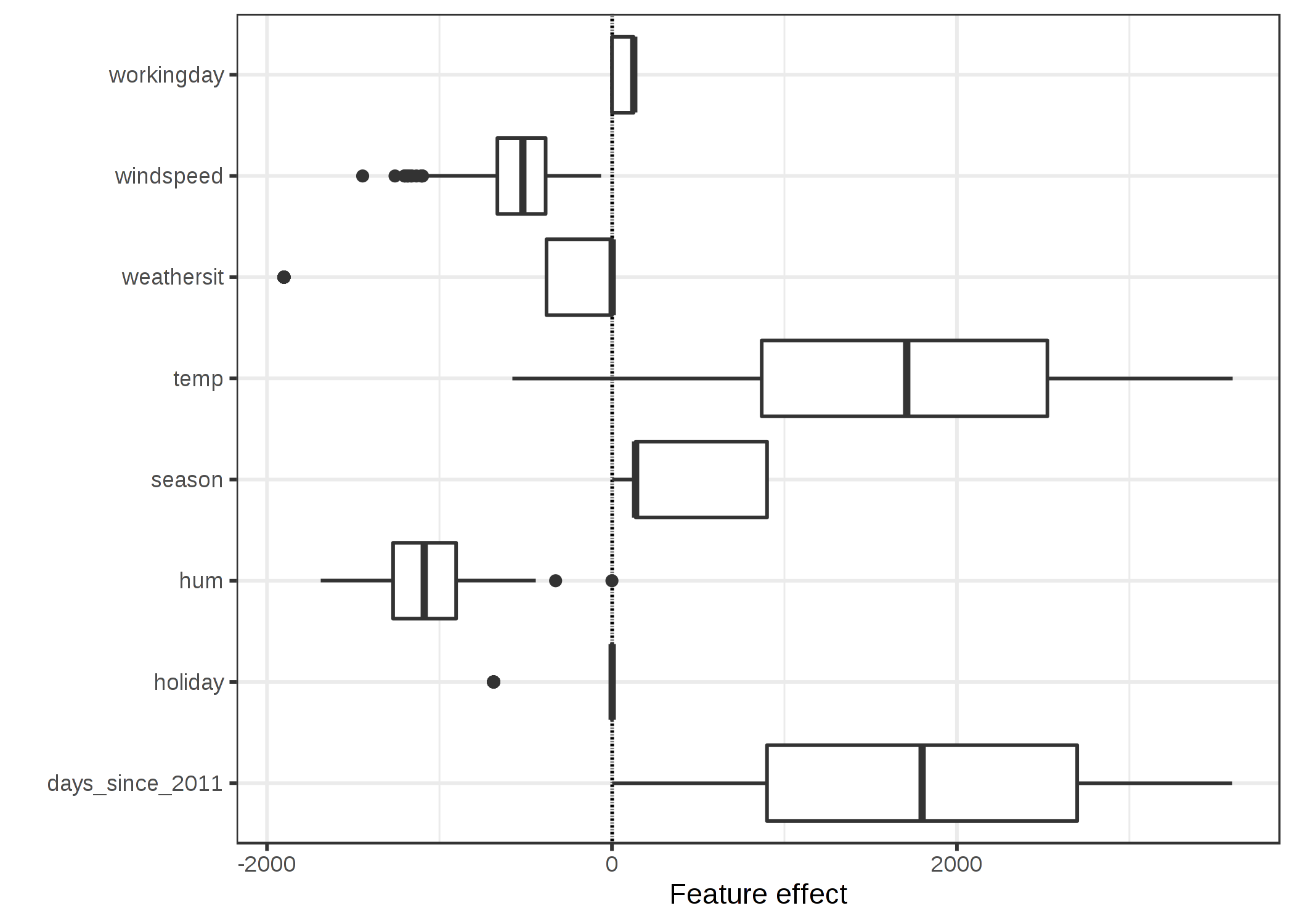
ภาพประกอบ 4.2: The feature effect plot shows the distribution of effects (= feature value times feature weight) across the data per feature.
The largest contributions to the expected number of rented bicycles comes from the temperature feature and the days feature, which captures the trend of bike rentals over time. The temperature has a broad range of how much it contributes to the prediction. The day trend feature goes from zero to large positive contributions, because the first day in the dataset (01.01.2011) has a very small trend effect and the estimated weight for this feature is positive (4.93). This means that the effect increases with each day and is highest for the last day in the dataset (31.12.2012). Note that for effects with a negative weight, the instances with a positive effect are those that have a negative feature value. For example, days with a high negative effect of windspeed are the ones with high wind speeds.
4.1.4 Explain Individual Predictions
How much has each feature of an instance contributed to the prediction? This can be answered by computing the effects for this instance. An interpretation of instance-specific effects only makes sense in comparison to the distribution of the effect for each feature. We want to explain the prediction of the linear model for the 6-th instance from the bicycle dataset. The instance has the following feature values.
| Feature | Value |
|---|---|
| season | SPRING |
| yr | 2011 |
| mnth | JAN |
| holiday | NO HOLIDAY |
| weekday | THU |
| workingday | WORKING DAY |
| weathersit | GOOD |
| temp | 1.604356 |
| hum | 51.8261 |
| windspeed | 6.000868 |
| cnt | 1606 |
| days_since_2011 | 5 |
To obtain the feature effects of this instance, we have to multiply its feature values by the corresponding weights from the linear regression model. For the value "WORKING DAY" of feature "workingday", the effect is, 124.9. For a temperature of 1.6 degrees Celsius, the effect is 177.6. We add these individual effects as crosses to the effect plot, which shows us the distribution of the effects in the data. This allows us to compare the individual effects with the distribution of effects in the data.
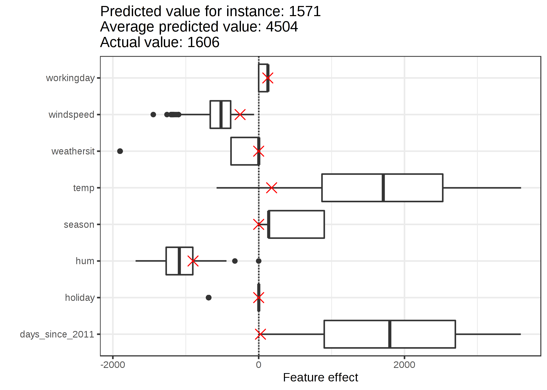
ภาพประกอบ 4.3: The effect plot for one instance shows the effect distribution and highlights the effects of the instance of interest.
If we average the predictions for the training data instances, we get an average of 4504. In comparison, the prediction of the 6-th instance is small, since only 1571 bicycle rents are predicted. The effect plot reveals the reason why. The boxplots show the distributions of the effects for all instances of the dataset, the crosses show the effects for the 6-th instance. The 6-th instance has a low temperature effect because on this day the temperature was 2 degrees, which is low compared to most other days (and remember that the weight of the temperature feature is positive). Also, the effect of the trend feature "days_since_2011" is small compared to the other data instances because this instance is from early 2011 (5 days) and the trend feature also has a positive weight.
4.1.5 Encoding of Categorical Features
There are several ways to encode a categorical feature, and the choice influences the interpretation of the weights.
The standard in linear regression models is treatment coding, which is sufficient in most cases. Using different encodings boils down to creating different (design) matrices from a single column with the categorical feature. This section presents three different encodings, but there are many more. The example used has six instances and a categorical feature with three categories. For the first two instances, the feature takes category A; for instances three and four, category B; and for the last two instances, category C.
Treatment coding
In treatment coding, the weight per category is the estimated difference in the prediction between the corresponding category and the reference category. The intercept of the linear model is the mean of the reference category (when all other features remain the same). The first column of the design matrix is the intercept, which is always 1. Column two indicates whether instance i is in category B, column three indicates whether it is in category C. There is no need for a column for category A, because then the linear equation would be overspecified and no unique solution for the weights can be found. It is sufficient to know that an instance is neither in category B or C.
Feature matrix: \[\begin{pmatrix}1&0&0\\1&0&0\\1&1&0\\1&1&0\\1&0&1\\1&0&1\\\end{pmatrix}\]
Effect coding
The weight per category is the estimated y-difference from the corresponding category to the overall mean (given all other features are zero or the reference category). The first column is used to estimate the intercept. The weight \(\beta_{0}\) associated with the intercept represents the overall mean and \(\beta_{1}\), the weight for column two, is the difference between the overall mean and category B. The total effect of category B is \(\beta_{0}+\beta_{1}\). The interpretation for category C is equivalent. For the reference category A, \(-(\beta_{1}+\beta_{2})\) is the difference to the overall mean and \(\beta_{0}-(\beta_{1}+\beta_{2})\) the overall effect.
Feature matrix: \[\begin{pmatrix}1&-1&-1\\1&-1&-1\\1&1&0\\1&1&0\\1&0&1\\1&0&1\\\end{pmatrix}\]
Dummy coding
The \(\beta\) per category is the estimated mean value of y for each category (given all other feature values are zero or the reference category). Note that the intercept has been omitted here so that a unique solution can be found for the linear model weights. Another way to mitigate this multicollinearity problem is to leave out one of the categories.
Feature matrix: \[\begin{pmatrix}1&0&0\\1&0&0\\0&1&0\\0&1&0\\0&0&1\\0&0&1\\\end{pmatrix}\]
If you want to dive a little deeper into the different encodings of categorical features, checkout this overview webpage and this blog post.
4.1.6 Do Linear Models Create Good Explanations?
Judging by the attributes that constitute a good explanation, as presented in the Human-Friendly Explanations chapter, linear models do not create the best explanations. They are contrastive, but the reference instance is a data point where all numerical features are zero and the categorical features are at their reference categories. This is usually an artificial, meaningless instance that is unlikely to occur in your data or reality. There is an exception: If all numerical features are mean centered (feature minus mean of feature) and all categorical features are effect coded, the reference instance is the data point where all the features take on the mean feature value. This might also be a non-existent data point, but it might at least be more likely or more meaningful. In this case, the weights times the feature values (feature effects) explain the contribution to the predicted outcome contrastive to the "mean-instance". Another aspect of a good explanation is selectivity, which can be achieved in linear models by using less features or by training sparse linear models. But by default, linear models do not create selective explanations. Linear models create truthful explanations, as long as the linear equation is an appropriate model for the relationship between features and outcome. The more non-linearities and interactions there are, the less accurate the linear model will be and the less truthful the explanations become. Linearity makes the explanations more general and simpler. The linear nature of the model, I believe, is the main factor why people use linear models for explaining relationships.
4.1.7 Sparse Linear Models
The examples of the linear models that I have chosen all look nice and neat, do they not? But in reality you might not have just a handful of features, but hundreds or thousands. And your linear regression models? Interpretability goes downhill. You might even find yourself in a situation where there are more features than instances, and you cannot fit a standard linear model at all. The good news is that there are ways to introduce sparsity (= few features) into linear models.
4.1.7.1 Lasso
Lasso is an automatic and convenient way to introduce sparsity into the linear regression model. Lasso stands for "least absolute shrinkage and selection operator" and, when applied in a linear regression model, performs feature selection and regularization of the selected feature weights. Let us consider the minimization problem that the weights optimize:
\[min_{\boldsymbol{\beta}}\left(\frac{1}{n}\sum_{i=1}^n(y^{(i)}-x_i^T\boldsymbol{\beta})^2\right)\]
Lasso adds a term to this optimization problem.
\[min_{\boldsymbol{\beta}}\left(\frac{1}{n}\sum_{i=1}^n(y^{(i)}-x_{i}^T\boldsymbol{\beta})^2+\lambda||\boldsymbol{\beta}||_1\right)\]
The term \(||\boldsymbol{\beta}||_1\), the L1-norm of the feature vector, leads to a penalization of large weights. Since the L1-norm is used, many of the weights receive an estimate of 0 and the others are shrunk. The parameter lambda (\(\lambda\)) controls the strength of the regularizing effect and is usually tuned by cross-validation. Especially when lambda is large, many weights become 0. The feature weights can be visualized as a function of the penalty term lambda. Each feature weight is represented by a curve in the following figure.
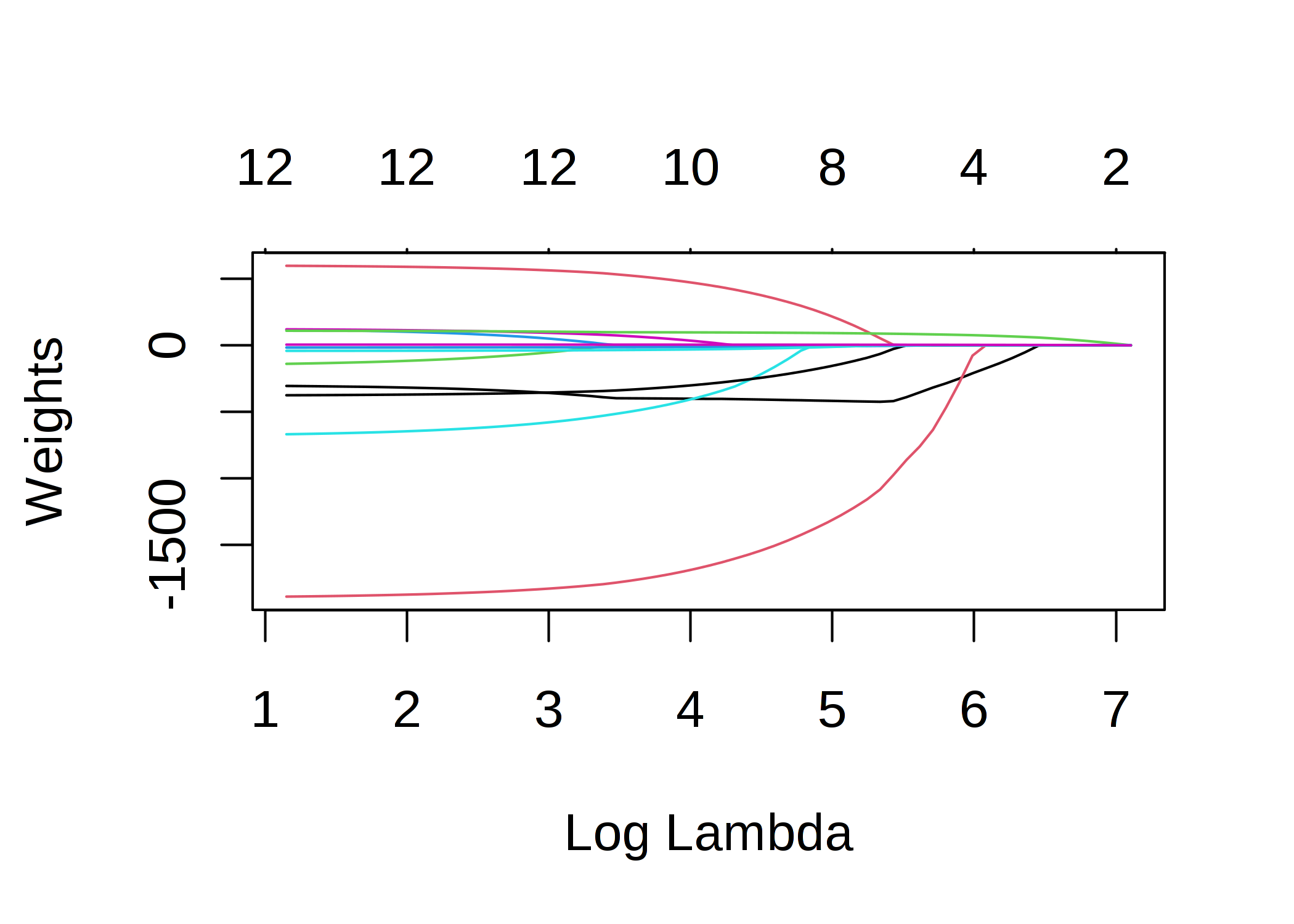
ภาพประกอบ 4.4: With increasing penalty of the weights, fewer and fewer features receive a non-zero weight estimate. These curves are also called regularization paths. The number above the plot is the number of non-zero weights.
What value should we choose for lambda? If you see the penalization term as a tuning parameter, then you can find the lambda that minimizes the model error with cross-validation. You can also consider lambda as a parameter to control the interpretability of the model. The larger the penalization, the fewer features are present in the model (because their weights are zero) and the better the model can be interpreted.
Example with Lasso
We will predict bicycle rentals using Lasso. We set the number of features we want to have in the model beforehand. Let us first set the number to 2 features:
| Weight | |
|---|---|
| seasonSPRING | 0.00 |
| seasonSUMMER | 0.00 |
| seasonFALL | 0.00 |
| seasonWINTER | 0.00 |
| holidayHOLIDAY | 0.00 |
| workingdayWORKING DAY | 0.00 |
| weathersitMISTY | 0.00 |
| weathersitRAIN/SNOW/STORM | 0.00 |
| temp | 52.33 |
| hum | 0.00 |
| windspeed | 0.00 |
| days_since_2011 | 2.15 |
The first two features with non-zero weights in the Lasso path are temperature ("temp") and the time trend ("days_since_2011").
Now, let us select 5 features:
| Weight | |
|---|---|
| seasonSPRING | -389.99 |
| seasonSUMMER | 0.00 |
| seasonFALL | 0.00 |
| seasonWINTER | 0.00 |
| holidayHOLIDAY | 0.00 |
| workingdayWORKING DAY | 0.00 |
| weathersitMISTY | 0.00 |
| weathersitRAIN/SNOW/STORM | -862.27 |
| temp | 85.58 |
| hum | -3.04 |
| windspeed | 0.00 |
| days_since_2011 | 3.82 |
Note that the weights for "temp" and "days_since_2011" differ from the model with two features. The reason for this is that by decreasing lambda even features that are already "in" the model are penalized less and may get a larger absolute weight. The interpretation of the Lasso weights corresponds to the interpretation of the weights in the linear regression model. You only need to pay attention to whether the features are standardized or not, because this affects the weights. In this example, the features were standardized by the software, but the weights were automatically transformed back for us to match the original feature scales.
Other methods for sparsity in linear models
A wide spectrum of methods can be used to reduce the number of features in a linear model.
Pre-processing methods:
- Manually selected features: You can always use expert knowledge to select or discard some features. The big drawback is that it cannot be automated and you need to have access to someone who understands the data.
- Univariate selection: An example is the correlation coefficient. You only consider features that exceed a certain threshold of correlation between the feature and the target. The disadvantage is that it only considers the features individually. Some features might not show a correlation until the linear model has accounted for some other features. Those ones you will miss with univariate selection methods.
Step-wise methods:
- Forward selection: Fit the linear model with one feature. Do this with each feature. Select the model that works best (e.g. highest R-squared). Now again, for the remaining features, fit different versions of your model by adding each feature to your current best model. Select the one that performs best. Continue until some criterion is reached, such as the maximum number of features in the model.
- Backward selection: Similar to forward selection. But instead of adding features, start with the model that contains all features and try out which feature you have to remove to get the highest performance increase. Repeat this until some stopping criterion is reached.
I recommend using Lasso, because it can be automated, considers all features simultaneously, and can be controlled via lambda. It also works for the logistic regression model for classification.
4.1.8 Advantages
The modeling of the predictions as a weighted sum makes it transparent how predictions are produced. And with Lasso we can ensure that the number of features used remains small.
Many people use linear regression models. This means that in many places it is accepted for predictive modeling and doing inference. There is a high level of collective experience and expertise, including teaching materials on linear regression models and software implementations. Linear regression can be found in R, Python, Java, Julia, Scala, Javascript, ...
Mathematically, it is straightforward to estimate the weights and you have a guarantee to find optimal weights (given all assumptions of the linear regression model are met by the data).
Together with the weights you get confidence intervals, tests, and solid statistical theory. There are also many extensions of the linear regression model (see chapter on GLM, GAM and more).
4.1.9 Disadvantages
Linear regression models can only represent linear relationships, i.e. a weighted sum of the input features. Each nonlinearity or interaction has to be hand-crafted and explicitly given to the model as an input feature.
Linear models are also often not that good regarding predictive performance, because the relationships that can be learned are so restricted and usually oversimplify how complex reality is.
The interpretation of a weight can be unintuitive because it depends on all other features. A feature with high positive correlation with the outcome y and another feature might get a negative weight in the linear model, because, given the other correlated feature, it is negatively correlated with y in the high-dimensional space. Completely correlated features make it even impossible to find a unique solution for the linear equation. An example: You have a model to predict the value of a house and have features like number of rooms and size of the house. House size and number of rooms are highly correlated: the bigger a house is, the more rooms it has. If you take both features into a linear model, it might happen, that the size of the house is the better predictor and gets a large positive weight. The number of rooms might end up getting a negative weight, because, given that a house has the same size, increasing the number of rooms could make it less valuable or the linear equation becomes less stable, when the correlation is too strong.
Friedman, Jerome, Trevor Hastie, and Robert Tibshirani. "The elements of statistical learning". www.web.stanford.edu/~hastie/ElemStatLearn/ (2009).↩