4.6 RuleFit
The RuleFit algorithm by Friedman and Popescu (2008)24 learns sparse linear models that include automatically detected interaction effects in the form of decision rules.
The linear regression model does not account for interactions between features. Would it not be convenient to have a model that is as simple and interpretable as linear models, but also integrates feature interactions? RuleFit fills this gap. RuleFit learns a sparse linear model with the original features and also a number of new features that are decision rules. These new features capture interactions between the original features. RuleFit automatically generates these features from decision trees. Each path through a tree can be transformed into a decision rule by combining the split decisions into a rule. The node predictions are discarded and only the splits are used in the decision rules:
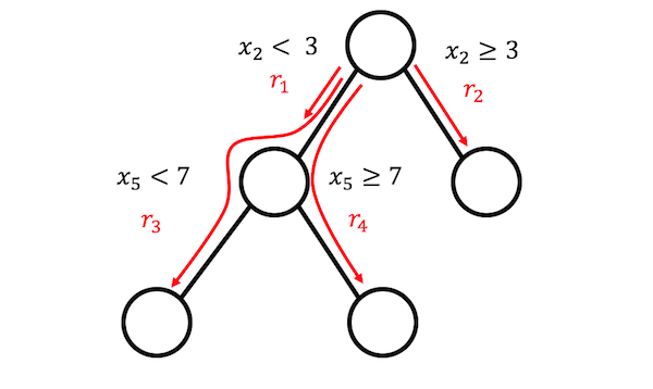
ภาพประกอบ 4.21: 4 rules can be generated from a tree with 3 terminal nodes.
Where do those decision trees come from? The trees are trained to predict the outcome of interest. This ensures that the splits are meaningful for the prediction task. Any algorithm that generates a lot of trees can be used for RuleFit, for example a random forest. Each tree is decomposed into decision rules that are used as additional features in a sparse linear regression model (Lasso).
The RuleFit paper uses the Boston housing data to illustrate this: The goal is to predict the median house value of a Boston neighborhood. One of the rules generated by RuleFit is: IF number of rooms > 6.64 AND concentration of nitric oxide <0.67 THEN 1 ELSE 0.
RuleFit also comes with a feature importance measure that helps to identify linear terms and rules that are important for the predictions. Feature importance is calculated from the weights of the regression model. The importance measure can be aggregated for the original features (which are used in their "raw" form and possibly in many decision rules).
RuleFit also introduces partial dependence plots to show the average change in prediction by changing a feature. The partial dependence plot is a model-agnostic method that can be used with any model, and is explained in the book chapter on partial dependence plots.
4.6.1 Interpretation and Example
Since RuleFit estimates a linear model in the end, the interpretation is the same as for "normal" linear models. The only difference is that the model has new features derived from decision rules. Decision rules are binary features: A value of 1 means that all conditions of the rule are met, otherwise the value is 0. For linear terms in RuleFit, the interpretation is the same as in linear regression models: If the feature increases by one unit, the predicted outcome changes by the corresponding feature weight.
In this example, we use RuleFit to predict the number of rented bicycles on a given day. The table shows five of the rules that were generated by RuleFit, along with their Lasso weights and importances. The calculation is explained later in the chapter.
| Description | Weight | Importance |
|---|---|---|
| days_since_2011 > 111 & weathersit in ("GOOD", "MISTY") | 793 | 303 |
| 37.25 <= hum <= 90 | -20 | 272 |
| temp > 13 & days_since_2011 > 554 | 676 | 239 |
| 4 <= windspeed <= 24 | -41 | 202 |
| days_since_2011 > 428 & temp > 5 | 366 | 179 |
The most important rule was: "days_since_2011 > 111 & weathersit in ("GOOD", "MISTY")" and the corresponding weight is 793. The interpretation is: If days_since_2011 > 111 & weathersit in ("GOOD", "MISTY"), then the predicted number of bikes increases by 793, when all other feature values remain fixed. In total, 278 such rules were created from the original 8 features. Quite a lot! But thanks to Lasso, only 58 of the 278 have a weight different from 0.
Computing the global feature importances reveals that temperature and time trend are the most important features:
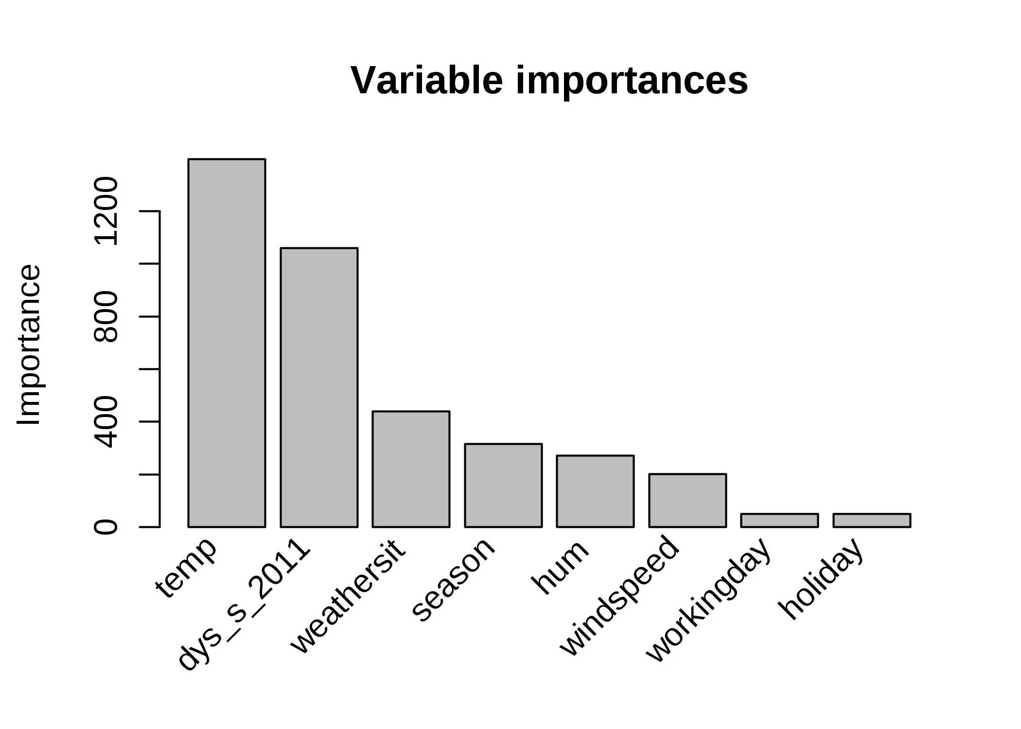
ภาพประกอบ 4.22: Feature importance measures for a RuleFit model predicting bike counts. The most important features for the predictions were temperature and time trend.
The feature importance measurement includes the importance of the raw feature term and all the decision rules in which the feature appears.
Interpretation template
The interpretation is analogous to linear models: The predicted outcome changes by \(\beta_j\) if feature \(x_j\) changes by one unit, provided all other features remain unchanged. The weight interpretation of a decision rule is a special case: If all conditions of a decision rule \(r_k\) apply, the predicted outcome changes by \(\alpha_k\) (the learned weight of rule \(r_k\) in the linear model).
For classification (using logistic regression instead of linear regression): If all conditions of the decision rule \(r_k\) apply, the odds for event vs. no-event changes by a factor of \(\alpha_k\).
4.6.2 Theory
Let us dive deeper into the technical details of the RuleFit algorithm. RuleFit consists of two components: The first component creates "rules" from decision trees and the second component fits a linear model with the original features and the new rules as input (hence the name "RuleFit").
Step 1: Rule generation
What does a rule look like? The rules generated by the algorithm have a simple form. For example: IF x2 < 3 AND x5 < 7 THEN 1 ELSE 0. The rules are constructed by decomposing decision trees: Any path to a node in a tree can be converted to a decision rule. The trees used for the rules are fitted to predict the target outcome. Therefore the splits and resulting rules are optimized to predict the outcome you are interested in. You simply chain the binary decisions that lead to a certain node with "AND", and voilà, you have a rule. It is desirable to generate a lot of diverse and meaningful rules. Gradient boosting is used to fit an ensemble of decision trees by regressing or classifying y with your original features X. Each resulting tree is converted into multiple rules. Not only boosted trees, but any tree ensemble algorithm can be used to generate the trees for RuleFit. A tree ensemble can be described with this general formula:
\[f(x)=a_0+\sum_{m=1}^M{}a_m{}f_m(X)\]
M is the number of trees and \(f_m(x)\) is the prediction function of the m-th tree. The \(a\)'s are the weights. Bagged ensembles, random forest, AdaBoost and MART produce tree ensembles and can be used for RuleFit.
We create the rules from all trees of the ensemble. Each rule \(r_m\) takes the form of:
\[r_m(x)=\prod_{j\in\text{T}_m}I(x_j\in{}s_{jm})\]
where \(\text{T}_{m}\) is the set of features used in the m-th tree, I is the indicator function that is 1 when feature \(x_j\) is in the specified subset of values s for the j-th feature (as specified by the tree splits) and 0 otherwise. For numerical features, \(s_{jm}\) is an interval in the value range of the feature. The interval looks like one of the two cases:
\[x_{s_{jm},\text{lower}}<x_j\]
\[x_j<x_{s_{jm},upper}\]
Further splits in that feature possibly lead to more complicated intervals. For categorical features the subset s contains some specific categories of the feature.
A made up example for the bike rental dataset:
\[r_{17}(x)=I(x_{\text{temp}}<15)\cdot{}I(x_{\text{weather}}\in\{\text{good},\text{cloudy}\})\cdot{}I(10\leq{}x_{\text{windspeed}}<20)\]
This rule returns 1 if all three conditions are met, otherwise 0. RuleFit extracts all possible rules from a tree, not only from the leaf nodes. So another rule that would be created is:
\[r_{18}(x)=I(x_{\text{temp}}<15)\cdot{}I(x_{\text{weather}}\in\{\text{good},\text{cloudy}\}\]
Altogether, the number of rules created from an ensemble of M trees with \(t_m\) terminal nodes each is:
\[K=\sum_{m=1}^M2(t_m-1)\]
A trick introduced by the RuleFit authors is to learn trees with random depth so that many diverse rules with different lengths are generated. Note that we discard the predicted value in each node and only keep the conditions that lead us to a node and then we create a rule from it. The weighting of the decision rules is done in step 2 of RuleFit.
Another way to see step 1: RuleFit generates a new set of features from your original features. These features are binary and can represent quite complex interactions of your original features. The rules are chosen to maximize the prediction task. The rules are automatically generated from the covariates matrix X. You can simply see the rules as new features based on your original features.
Step 2: Sparse linear model
You get MANY rules in step 1. Since the first step can be seen as only a feature transformation, you are still not done with fitting a model. Also, you want to reduce the number of rules. In addition to the rules, all your "raw" features from your original dataset will also be used in the sparse linear model. Every rule and every original feature becomes a feature in the linear model and gets a weight estimate. The original raw features are added because trees fail at representing simple linear relationships between y and x. Before we train a sparse linear model, we winsorize the original features so that they are more robust against outliers:
\[l_j^*(x_j)=min(\delta_j^+,max(\delta_j^-,x_j))\]
where \(\delta_j^-\) and \(\delta_j^+\) are the \(\delta\) quantiles of the data distribution of feature \(x_j\). A choice of 0.05 for \(\delta\) means that any value of feature \(x_j\) that is in the 5% lowest or 5% highest values will be set to the quantiles at 5% or 95% respectively. As a rule of thumb, you can choose \(\delta\) = 0.025. In addition, the linear terms have to be normalized so that they have the same prior importance as a typical decision rule:
\[l_j(x_j)=0.4\cdot{}l^*_j(x_j)/std(l^*_j(x_j))\]
The \(0.4\) is the average standard deviation of rules with a uniform support distribution of \(s_k\sim{}U(0,1)\).
We combine both types of features to generate a new feature matrix and train a sparse linear model with Lasso, with the following structure:
\[\hat{f}(x)=\hat{\beta}_0+\sum_{k=1}^K\hat{\alpha}_k{}r_k(x)+\sum_{j=1}^p\hat{\beta}_j{}l_j(x_j)\]
where \(\hat{\alpha}\) is the estimated weight vector for the rule features and \(\hat{\beta}\) the weight vector for the original features. Since RuleFit uses Lasso, the loss function gets the additional constraint that forces some of the weights to get a zero estimate:
\[(\{\hat{\alpha}\}_1^K,\{\hat{\beta}\}_0^p)=argmin_{\{\hat{\alpha}\}_1^K,\{\hat{\beta}\}_0^p}\sum_{i=1}^n{}L(y^{(i)},f(x^{(i)}))+\lambda\cdot\left(\sum_{k=1}^K|\alpha_k|+\sum_{j=1}^p|b_j|\right)\]
The result is a linear model that has linear effects for all of the original features and for the rules. The interpretation is the same as for linear models, the only difference is that some features are now binary rules.
Step 3 (optional): Feature importance
For the linear terms of the original features, the feature importance is measured with the standardized predictor:
\[I_j=|\hat{\beta}_j|\cdot{}std(l_j(x_j))\]
where \(\beta_j\) is the weight from the Lasso model and \(std(l_j(x_j))\) is the standard deviation of the linear term over the data.
For the decision rule terms, the importance is calculated with the following formula:
\[I_k=|\hat{\alpha}_k|\cdot\sqrt{s_k(1-s_k)}\]
where \(\hat{\alpha}_k\) is the associated Lasso weight of the decision rule and \(s_k\) is the support of the feature in the data, which is the percentage of data points to which the decision rule applies (where \(r_k(x)=1\)):
\[s_k=\frac{1}{n}\sum_{i=1}^n{}r_k(x^{(i)})\]
A feature occurs as a linear term and possibly also within many decision rules. How do we measure the total importance of a feature? The importance \(J_j(x)\) of a feature can be measured for each individual prediction:
\[J_j(x)=I_j(x)+\sum_{x_j\in{}r_k}I_k(x)/m_k\]
where \(I_l\) is the importance of the linear term and \(I_k\) the importance of the decision rules in which \(x_j\) appears, and \(m_k\) is the number of features constituting the rule \(r_k\). Adding the feature importance from all instances gives us the global feature importance:
\[J_j(X)=\sum_{i=1}^n{}J_j(x^{(i)})\]
It is possible to select a subset of instances and calculate the feature importance for this group.
4.6.3 Advantages
RuleFit automatically adds feature interactions to linear models. Therefore, it solves the problem of linear models that you have to add interaction terms manually and it helps a bit with the issue of modeling nonlinear relationships.
RuleFit can handle both classification and regression tasks.
The rules created are easy to interpret, because they are binary decision rules. Either the rule applies to an instance or not. Good interpretability is only guaranteed if the number of conditions within a rule is not too large. A rule with 1 to 3 conditions seems reasonable to me. This means a maximum depth of 3 for the trees in the tree ensemble.
Even if there are many rules in the model, they do not apply to every instance. For an individual instance only a handful of rules apply (= have a non-zero weights). This improves local interpretability.
RuleFit proposes a bunch of useful diagnostic tools. These tools are model-agnostic, so you can find them in the model-agnostic section of the book: feature importance, partial dependence plots and feature interactions.
4.6.4 Disadvantages
Sometimes RuleFit creates many rules that get a non-zero weight in the Lasso model. The interpretability degrades with increasing number of features in the model. A promising solution is to force feature effects to be monotonic, meaning that an increase of a feature has to lead to an increase of the prediction.
An anecdotal drawback: The papers claim a good performance of RuleFit -- often close to the predictive performance of random forests! -- but in the few cases where I tried it personally, the performance was disappointing. Just try it out for your problem and see how it performs.
The end product of the RuleFit procedure is a linear model with additional fancy features (the decision rules). But since it is a linear model, the weight interpretation is still unintuitive. It comes with the same "footnote" as a usual linear regression model: "... given all features are fixed." It gets a bit more tricky when you have overlapping rules. For example, one decision rule (feature) for the bicycle prediction could be: "temp > 10" and another rule could be "temp > 15 & weather='GOOD'". If the weather is good and the temperature is above 15 degrees, the temperature is automatically greater then 10. In the cases where the second rule applies, the first rule applies as well. The interpretation of the estimated weight for the second rule is: "Assuming all other features remain fixed, the predicted number of bikes increases by \(\beta_2\) when the weather is good and temperature above 15 degrees.". But, now it becomes really clear that the 'all other feature fixed' is problematic, because if rule 2 applies, also rule 1 applies and the interpretation is nonsensical.
4.6.5 Software and Alternative
The RuleFit algorithm is implemented in R by Fokkema and Christoffersen (2017)25 and you can find a Python version on Github.
A very similar framework is skope-rules, a Python module that also extracts rules from ensembles. It differs in the way it learns the final rules: First, skope-rules remove low-performing rules, based on recall and precision thresholds. Then, duplicate and similar rules are removed by performing a selection based on the diversity of logical terms (variable + larger/smaller operator) and performance (F1-score) of the rules. This final step does not rely on using Lasso, but considers only the out-of-bag F1-score and the logical terms which form the rules.
Friedman, Jerome H, and Bogdan E Popescu. "Predictive learning via rule ensembles." The Annals of Applied Statistics. JSTOR, 916–54. (2008).↩
Fokkema, Marjolein, and Benjamin Christoffersen. "Pre: Prediction rule ensembles". https://CRAN.R-project.org/package=pre (2017).↩