7.2 Pixel Attribution (Saliency Maps)
This chapter is currently only available in this web version. ebook and print will follow.
Pixel attribution methods highlight the pixels that were relevant for a certain image classification by a neural network. The following image is an example of an explanation:
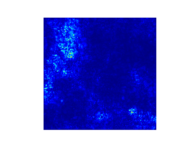
You will see later in this chapter what is going on in this particular image. Pixel attribution methods can be found under various names: sensitivity map, saliency map, pixel attribution map, gradient-based attribution methods, feature relevance, feature attribution, and feature contribution.
Pixel attribution is a special case of feature attribution, but for images. Feature attribution explains individual predictions by attributing each input feature according to how much it changed the prediction (negatively or positively). The features can be input pixels, tabular data or words. SHAP, Shapley Values and LIME are examples of general feature attribution methods.
We consider neural networks that output as prediction a vector of length \(C\), which includes regression where \(C=1\). The output of the neural network for image I is called \(S(I)=[S_1(I),\ldots,S_C(I)]\). All these methods take as input \(x\in\mathbb{R}^p\) (can be image pixels, tabular data, words, ...) with p features and output as explanation a relevance value for each of the p input features: \(R^c=[R_1^c,\ldots,R_p^c]\). The c indicates the relevance for the c-th output \(S_C(I)\).
There is a confusing amount of pixel attribution approaches. It helps to understand that there are two different types of attribution methods:
Occlusion- or perturbation-based: Methods like SHAP and LIME manipulate parts of the image to generate explanations (model-agnostic).
Gradient-based: Many methods compute the gradient of the prediction (or classification score) with respect to the input features. The gradient-based methods (of which there are many) mostly differ in how the gradient is computed.
Both approaches have in common that the explanation has the same size as the input image (or at least can be meaningfully projected onto it) and they assign each pixel a value that can be interpreted as the relevance of the pixel to the prediction or classification of that image.
Another useful categorization for pixel attribution methods is the baseline question:
Gradient-only methods tell us whether a change in a pixel would change the prediction. Examples are Vanilla Gradient and Grad-CAM. The interpretation of the gradient-only attribution is: If I were to change this pixel, the predicted class probability would go up (for positive gradient) or down (for negative gradient). The larger the absolute value of the gradient, the stronger the effect of a change at this pixel.
Path-attribution methods compare the current image to a reference image, which can be an artificial "zero" image such as a completely grey image. The difference in actual and baseline prediction is divided among the pixels. The baseline image can also be multiple images: a distribution of images. This category includes model-specific gradient-based methods such as Deep Taylor and Integrated Gradients, as well as model-agnostic methods such as LIME and SHAP. Some path attribution methods are "complete", meaning that the sum of the relevance values for all input features is the difference between the prediction of the image minus the prediction of a reference image. Examples are SHAP and Integrated Gradients. For path-attribution methods, the interpretation is always done with respect to the baseline: The difference between classification scores of the actual image and the baseline image are attributed to the pixels. The choice of the reference image (distribution) has a big effect on the explanation. The usual assumption is to use a "neutral" image (distribution). Of course, it is perfectly possible to use your favorite selfie, but you should ask yourself if it makes sense in an application. It would certainly assert dominance among the other project members.
Add this point I would normally give an intuition about how these methods work, but I think it is best if we just start with the Vanilla Gradient method, because it shows very nicely the general recipe that many other methods follow.
7.2.1 Vanilla Gradient (Saliency Maps)
The idea of Vanilla Gradient, introduced by 81 as one of the first pixel attribution approaches is quite simple if you already know backpropagation. (They called their approach "Image-Specific Class Saliency", but I like Vanilla Gradient better). We calculate the gradient of the loss function for the class we are interested in with respect to the input pixels. This gives us a map of the size of the input features with negative to positive values.
The recipe for this approach is:
- Perform a forward pass of the image of interest.
- Compute the gradient of class score of interest with respect to the input pixels: \[E_{grad}(I_0)=\frac{\delta{}S_c}{\delta{}I}|_{I=I_0}\] Here we set all other classes to zero.
- Visualize the gradients. You can either show the absolute values or highlight negative and positive contributions separately.
More formally, we have an image I and the convolutional neural network gives it a score \(S_c(I)\) for class c. The score is a highly non-linear function of our image. The idea behind using the gradient is that we can approximate that score by applying a first-order Taylor expansion
\[S_c(I)\approx{}w^T{}I+b\]
where w is the derivate of our score:
\[w = \frac{\delta S_C}{\delta I}|_{I_0}\]
Now, there is some ambiguity how to perform a backward pass of the gradients, since non-linear units such as ReLU (Rectifying Linear Unit) "remove" the sign. So when we do a backpass, we do not know whether to assign a positive or negative activation. Using my incredible ASCII art skill, the ReLU function looks like this: _/ and is defined as \(X_{n+1}(x)=max(0,X_n)\) from layer \(X_n\) to layer \(X_{n-1}\). This means that when the activation of a neuron is 0, we do not know which value to backpropagate. In the case of Vanilla Gradient, the ambiguity is resolved as follows:
\[\frac{\delta f}{\delta X_n} = \frac{\delta f}{\delta X_{n+1}} \cdot \mathbf{I}(X_n > 0)\]
Here, \(\mathbf{I}\) is the element-wise indicator function, which is 0 where the activation at the lower layer was negative, and 1 where it is positive or zero. Vanilla Gradient takes the gradient we have back-propagated so far up to layer n+1, and then simply sets the gradients to zero where the activation at the layer below is negative.
Let us look at an example where we have layers \(X_n\) and \(X_{n+1}=ReLU(X_{n+1})\). Our fictive activation at \(X_n\) is:
\[ \begin{pmatrix} 1 & 0 \\ -1 & -10 \\ \end{pmatrix} \]
And these are our gradients at \(X_{(n+1)}\):
\[ \begin{pmatrix} 0.4 & 1.1 \\ -0.5 & -0.1 \\ \end{pmatrix} \]
Then our gradients at \(X_n\) are:
\[ \begin{pmatrix} 0.4 & 0 \\ 0 & 0 \\ \end{pmatrix} \]
7.2.1.1 Problems with Vanilla Gradient
Vanilla Gradient has a saturation problem (explained in Avanti et. al, 2017 82): When ReLU is used, and when the activation goes below zero, then the activation is capped at zero and does not change any more. The activation is saturated. For example: The input to the layer is two neurons with weights \(-1\) and \(-1\) and a bias of \(1\). When passing through the ReLU layer, the activation will be neuron1 + neuron2 if the sum of both neurons is less than 1. If the sum of both is greater than 1, the activation will remain saturated at an activation of 1. Also the gradient at this point will be zero, and Vanilla Gradient will say that this neuron is not important.
And now, my dear readers, learn another method, more or less for free: DeconvNet
7.2.2 DeconvNet
DeconvNet by Zeiler an Fergus (2014) 83 is almost identical to Vanilla Gradient. The goal of DeconvNet is to reverse a neural network and the paper proposes operations that are reversals of the filtering, pooling and activation layers. If you take a look into the paper, it looks very different to Vanilla Gradient, but apart from the reversal of the ReLU layer, DeconvNet is equivalent to the Vanilla Gradient approach. Vanilla Gradient can be seen as a generalization of DeconvNet. DeconvNet makes a different choice for backpropagating the gradient through ReLU:
\(R_n=R_{n+1}\mathbb{I}(R_{n+1}>0)\)$,
where \(R_n\) and \(R_{n+1}\) are the layer reconstructions. When backpassing from layer n to layer n-1, DeconvNet "remembers" which of the activations in layer n were set to zero in the forward pass and sets them to 0 in layer n-1. Activations with a negative value in layer x are set to zero in layer n-1. The gradient \(X_n\) for the example from earlier becomes:
\[ \begin{pmatrix} 0.4 & 1.1 \\ 0 & 0 \\ \end{pmatrix} \]
7.2.3 Grad-CAM
Grad-CAM provides visual explanations for CNN decisions. Unlike other methods, the gradient is not backpropagated all the way back to the image, but (usually) to the last convolutional layer to produce a coarse localization map that highlights important regions of the image.
Grad-CAM stands for Gradient-weighted Class Activation Map. And, as the name suggests, it is based on the gradient of the neural networks. Grad-CAM, like other techniques, assigns each neuron a relevance score for the decision of interest. This decision of interest can be the class prediction (which we find in the output layer), but can theoretically be any other layer in the neural network. Grad-CAM backpropagates this information to the last convolutional layer. Grad-CAM can be used with different CNNs: with fully-connected layers, for structured output such as captioning and in multi-task outputs, and for reinforcement learning.
Let us start with an intuitive consideration of Grad-CAM. The goal of Grad-CAM is to understand at which parts of an image a convolutional layer "looks" for a certain classification. As a reminder, the first convolutional layer of a CNN takes as input the images and outputs feature maps that encode learned features (see the chapter on Learned Features). The higher-level convolutional layers do the same, but take as input the feature maps of the previous convolutional layers. To understand how the CNN makes decisions, Grad-CAM analyzes which regions are activated in the feature maps of the last convolutional layers. There are k feature maps in the last convolutional layer, and I will call them \(A_1, A_2, \ldots, A_k\). How can we "see" from the feature maps how the convolutional neural network has made a certain classification? In the first approach, we could simply visualize the raw values of each feature map, average over the feature maps and overlay this over our image. This would not be helpful since the feature maps encode information for all classes, but we are interested in a particular class. Grad-CAM has to decide how important each of the k feature map was to our class c that we are interested in. We have to weight each pixel of each feature map with the gradient before we average over the feature maps. This give us a heatmap which highlights regions that positively or negatively affect the class of interest. This heatmap is send through the ReLU function, which is a fancy way of saying that we set all negative values to zero. Grad-CAM removes all negative values by using a ReLU function, with the argument that we are only interested in the parts that contribute to the selected class c and not to other classes. The word pixel might be misleading here as the feature map is smaller than the image (because of the pooling units) but is mapped back to the original image. We then scale the Grad-CAM map to the interval [0,1] for visualization purposes and overlay it over the original image.
Let us look at the recipe for Grad-CAM Our goal is to find the localization map, which is defined as:
\[L^c_{Grad-CAM} \in \mathbb{R}^{u\times v} = \underbrace{ReLU}_{\text{Pick positive values}}\left(\sum_{k} \alpha_k^c A^k\right)\]
Here, u is the width, v the height of the explanation and c the class of interest.
- Forward propagate the input image through the convolutional neural network.
- Obtain the raw score for the class of interest, meaning the activation of the neuron before the softmax layer.
- Set all other class activations to zero.
- Backpropagate the gradient of the class of interest to the last convolutional layer before the fully connected layers: \(\frac{\delta{}y^c}{\delta{}A^k}\).
- Weight each feature map "pixel" by the gradient for the class. Indices i and j refer to the width and height dimensions: \[\alpha_k^c = \overbrace{\frac{1}{Z}\sum_{i}\sum_{j}}^{\text{global average pooling}} \underbrace{\frac{\delta y^c}{\delta A_{ij}^k}}_{\text{gradients via backprop}}\] This means that the gradients are globally pooled.
- Calculate an average of the feature maps, weighted per pixel by the gradient.
- Apply ReLU to the averaged feature map.
- For visualization: Scale values to the interval between 0 and 1. Upscale the image and overlay it over the original image.
- Additional step for Guided Grad-CAM: Multiply heatmap with guided backpropagation.
7.2.4 Guided Grad-CAM
From the description of Grad-CAM you can guess that the localization is very coarse since the last convolutional feature maps have a much coarser resolution compared to the input image. In contrast, other attribution techniques backpropagate all the way to the input pixels. They are therefore much more detailed and can show you individual edges or spots that contributed most to a prediction. A fusion of both methods is called Guided Grad-CAM. And it is super simple. You compute for an image both the Grad-CAM explanation and the explanation from another attribution method, such as Vanilla Gradient. The Grad-CAM output is then upsampled with bilinear interpolation, then both maps are multiplied element-wise. Grad-CAM works like a lense that focuses on specific parts of the pixel-wise attribution map.
7.2.5 SmoothGrad
The idea of SmoothGrad by Smilkov et. al 2017 84 is to make gradient-based explanations less noisy by adding noise and averaging over these artificially noisy gradients. SmoothGrad is not an standalone explanation method, but an extension to any gradient-based explanation method.
SmoothGrad works in the following way:
- Generate multiple versions of the image of interest by adding noise to it.
- Create pixel attribution maps for all images.
- Average the pixel attribution maps.
Yes, it is that simple. Why should this work? The theory is that the derivative fluctuates greatly at small scales. Neural networks have no incentive during training to keep the gradients smooth, their goal is to classify images correctly. Averaging over multiple maps "smooths out" these fluctuations:
\[R_{sg}(x)=\frac{1}{N}\sum_{i=1}^n{}R(x+g_i),\]
Here, \(g_i\sim{}N(0,\sigma^2)\) are noise vectors sampled from the Gaussian distribution. The "ideal" noise level depends on the input image and the network. The authors suggest a noise level of 10%-20%, which means that \(\frac{\sigma}{x_{max} - x_{min}}\) should be between 0.1 and 0.2. The limits \(x_{max}\) and \(x_{min}\) refer to minimum and maximum pixel values of the image. The other parameter is the number of samples n, for which was suggested to use n = 50, since there are diminishing returns above that.
7.2.6 Examples
Let us see some examples of what these maps look like and how the methods compare qualitatively. The network under examination is VGG-16 (Simonyan et. al 2014 85) which was trained on ImageNet and can therefore distinguish more than 20,000 classes. For the following images we will create explanations for the class with the highest classification score.
These are the images and their classification by the neural network:
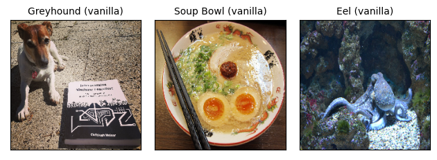
The image on the left with the honorable dog guarding the Interpretable Machine Learning book was classified as "Greyhound" with a probability of 35% (seems like "Interpretable Machine Learning book" was not one of the 20k classes). The image in the middle shows a bowl of yummy ramen soup and is correctly classified as "Soup Bowl" with a probability of 50%. The third image shows an octopus on the ocean floor, which is incorrectly classified as "Eel" with a high probability of 70%.
And these are the pixel attributions that aim to explain the classification:
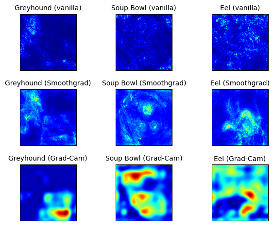
Unfortunately, it is a bit of a mess. But let us look at the individual explanations, starting with the dog. Vanilla Gradient and Vanilla Gradient + SmoothGrad both highlight the dog, which makes sense. But they also highlight some areas around the book, which is odd. Grad-CAM highlights only the book area, which makes no sense at all. And from here on, it gets a bit messier. The Vanilla Gradient method seems to fail for both the soup bowl and the octopus (or, as the network thinks, eel). Both images look like afterimages from looking into the sun for too long. (Please do not look at the sun directly). SmoothGrad helps a lot, at least the areas are more defined. In the soup example, some of the ingredients are highlighted, such as the eggs and the meat, but also the area around the chop sticks. In the octopus image, mostly the animal itself is highlighted.
For the soup bowl, Grad-CAM highlights the egg part and, for some reason, the upper part of the bowl. The octopus explanations by Grad-CAM are even messier.
You can already see here the difficulties in assessing whether we trust the explanations. As a first step, we need to consider which parts of the image contain information that is relevant to the images classification. But then we also need to think about what the neural network might have used for the classification. Perhaps the soup bowl was correctly classified based on the combination of eggs and chopstick, as SmoothGrad implies? Or maybe the neural network recognized the shape of the bow plus some ingredients, as Grad-CAM suggests? We just do not know.
And that is the big issue with all of these methods. We do not have a ground truth for the explanations. We can only, in a first step, reject explanations that obviously make no sense (and even in this step we don't have strong confidence. The prediction process in the neural network is very complicated).
7.2.7 Advantages
The explanations are visual and we are quick to recognize images. In particular, when methods only highlight important pixels, it is easy to immediately recognize the important regions of the image.
Gradient-based methods are usually faster to compute than model-agnostic methods. For example, LIME and SHAP can also be used to explain image classifications, but are more expensive to compute.
There are many methods to choose from.
7.2.8 Disadvantages
As with most interpretation methods, it is difficult to know whether an explanation is correct, and a huge part of the evaluation is only qualitative ("These explanations look about right, let's publish the paper already.").
Pixel attribution methods can be very fragile. Ghorbani et. al (2019)86 showed that introducing small (adversarial) perturbations to an image, that still lead to the same prediction, can lead to very different pixels being highlighted as explanations.
Kindermanns et. al (2019) 87 also showed that these pixel attribution methods can be highly unreliable. They added a constant shift to the input data, meaning they added the same pixel changes to all images. They compared two networks, the original network and "shifted" network where the bias of the first layer is changed to adapt for the constant pixel shift. Both networks produce the same predictions. Also the gradient is the same for both. But the explanations changed, which is an undesirable property. They looked at DeepLift, Vanilla Gradient and Integrated Gradients.
The paper "Sanity Checks for Saliency Maps" 88 investigated whether saliency methods are insensitive to model and data. Insensitivity is highly undesirable because it would mean that the "explanation" is unrelated to model and data. Methods that are insensitive to model and training data are similar to edge detectors. Edge detectors simply highlight strong pixel color changes in images and are unrelated to a prediction model or abstract features of the image, and require not training. The methods tested were Vanilla Gradient, Gradient x Input, Integrated Gradients, Guided Backpropagation, Guided Grad-CAM and SmoothGrad (with vanilla gradient). Vanilla gradients and Grad-CAM passed the insensitivity check, while Guided Backpropagation and Guided GradCAM fail. However, the sanity checks paper itself has found some criticism from Tomsett et. al (2020) 89 with a paper called "Sanity Checks for Saliency Metrics" (of course). They found that there is a lack of consistency for evaluation metrics (I know, it is getting pretty meta now). So we are back to where we started ... It remains difficult to evaluate the visual explanations. This makes it very difficult for a practitioner.
All in all, this is a very unsatisfactory state of affairs. We have to wait a little bit for more research on this topic. And please, no more invention of new methods, but more scrutiny of how to evaluate these methods.
7.2.9 Software
There are several software implementations of pixel attribution methods. For the example, I used tf-keras-vis. One of the most comprehensive libraries is iNNvestigate, which implements Vanilla gradient, Smoothgrad, Deconvnet, Guided Backpropagation, PatternNet, LRP and more. A lot of the methods are implemented in the DeepExplain Toolbox.
Simonyan, Karen, Andrea Vedaldi, and Andrew Zisserman. "Deep inside convolutional networks: Visualising image classification models and saliency maps." arXiv preprint arXiv:1312.6034 (2013).↩
Shrikumar, Avanti, Peyton Greenside, and Anshul Kundaje. "Learning important features through propagating activation differences." Proceedings of the 34th International Conference on Machine Learning-Volume 70. JMLR. org, (2017).↩
Zeiler, Matthew D., and Rob Fergus. "Visualizing and understanding convolutional networks." European conference on computer vision. Springer, Cham, 2014.↩
Smilkov, Daniel, et al. "Smoothgrad: removing noise by adding noise." arXiv preprint arXiv:1706.03825 (2017).↩
Simonyan, Karen, and Andrew Zisserman. "Very deep convolutional networks for large-scale image recognition." arXiv preprint arXiv:1409.1556 (2014).↩
Ghorbani, Amirata, Abubakar Abid, and James Zou. "Interpretation of neural networks is fragile." Proceedings of the AAAI Conference on Artificial Intelligence. Vol. 33. 2019.↩
Kindermans, Pieter-Jan, Sara Hooker, Julius Adebayo, Maximilian Alber, Kristof T. Schütt, Sven Dähne, Dumitru Erhan, and Been Kim. "The (un) reliability of saliency methods." In Explainable AI: Interpreting, Explaining and Visualizing Deep Learning, pp. 267-280. Springer, Cham, (2019).↩
Adebayo, Julius, Justin Gilmer, Michael Muelly, Ian Goodfellow, Moritz Hardt, and Been Kim. "Sanity checks for saliency maps." arXiv preprint arXiv:1810.03292 (2018).↩
Tomsett, Richard, Dan Harborne, Supriyo Chakraborty, Prudhvi Gurram, and Alun Preece. "Sanity checks for saliency metrics." In Proceedings of the AAAI Conference on Artificial Intelligence, vol. 34, no. 04, pp. 6021-6029. 2020.↩